
BART vs Causal forests showdown
Load packages
# library(devtools)
#devtools::install_github("vdorie/dbarts")
library(dbarts)
library(ggplot2)
library(tidyverse)
## ── Attaching packages ─────────────────────────────────────── tidyverse 1.3.0 ──## ✔ tibble 3.0.4 ✔ dplyr 1.0.2
## ✔ tidyr 1.1.2 ✔ stringr 1.4.0
## ✔ readr 1.4.0 ✔ forcats 0.5.0
## ✔ purrr 0.3.4## ── Conflicts ────────────────────────────────────────── tidyverse_conflicts() ──
## ✖ tidyr::extract() masks dbarts::extract()
## ✖ dplyr::filter() masks stats::filter()
## ✖ dplyr::lag() masks stats::lag()library(grf)
#devtools::install_github("vdorie/aciccomp/2017")
library(aciccomp2017)
library(cowplot)
source("CalcPosteriors.R")
fullrun <- 0Dataset 1: Simulated dataset from Friedman MARS paper
This is not a causal problem but a prediction problem.
## y = f(x) + epsilon , epsilon ~ N(0, sigma)
## x consists of 10 variables, only first 5 matter

f <- function(x) {
    10 * sin(pi * x[,1] * x[,2]) + 20 * (x[,3] - 0.5)^2 +
      10 * x[,4] + 5 * x[,5]
}

set.seed(99)
sigma <- 1.0
n     <- 100

x  <- matrix(runif(n * 10), n, 10)
Ey <- f(x)
y  <- rnorm(n, Ey, sigma)

df <- data.frame(x, y, y_true = Ey)
fit BART model on simulated Friedman data
if(fullrun){
## run BART
  set.seed(99)
  bartFit <- bart(x, y)
  saveRDS(bartFit, "s1.rds")
} else { bartFit <- readRDS("s1.rds")}

plot(bartFit)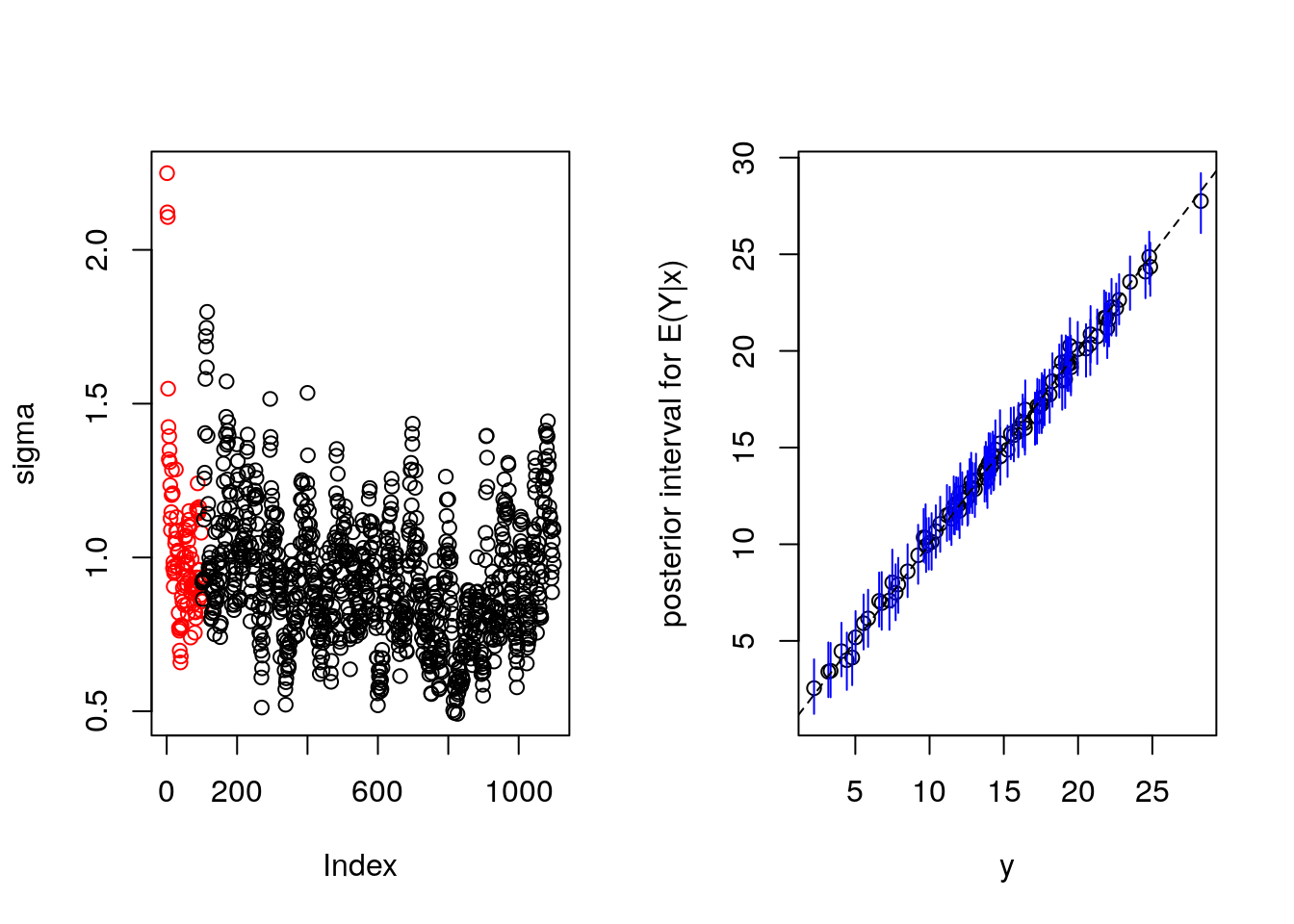
MCMC or sigma looks ok.
compare BART fit to true values
df2 <- data.frame(df,
  ql = apply(bartFit$yhat.train, length(dim(bartFit$yhat.train)), quantile,probs=0.05),
  qm = apply(bartFit$yhat.train, length(dim(bartFit$yhat.train)), quantile,probs=.5),
  qu <- apply(bartFit$yhat.train, length(dim(bartFit$yhat.train)), quantile,probs=0.95)
)

bartp <- ggplot(df2, aes(x= y, y = qm)) + geom_linerange(aes(ymin = ql, ymax = qu), col = "grey") +
  geom_point() + geom_smooth() +
  geom_abline(intercept = 0, slope = 1, col = "red", size = 1)

bartp
## `geom_smooth()` using method = 'loess' and formula 'y ~ x'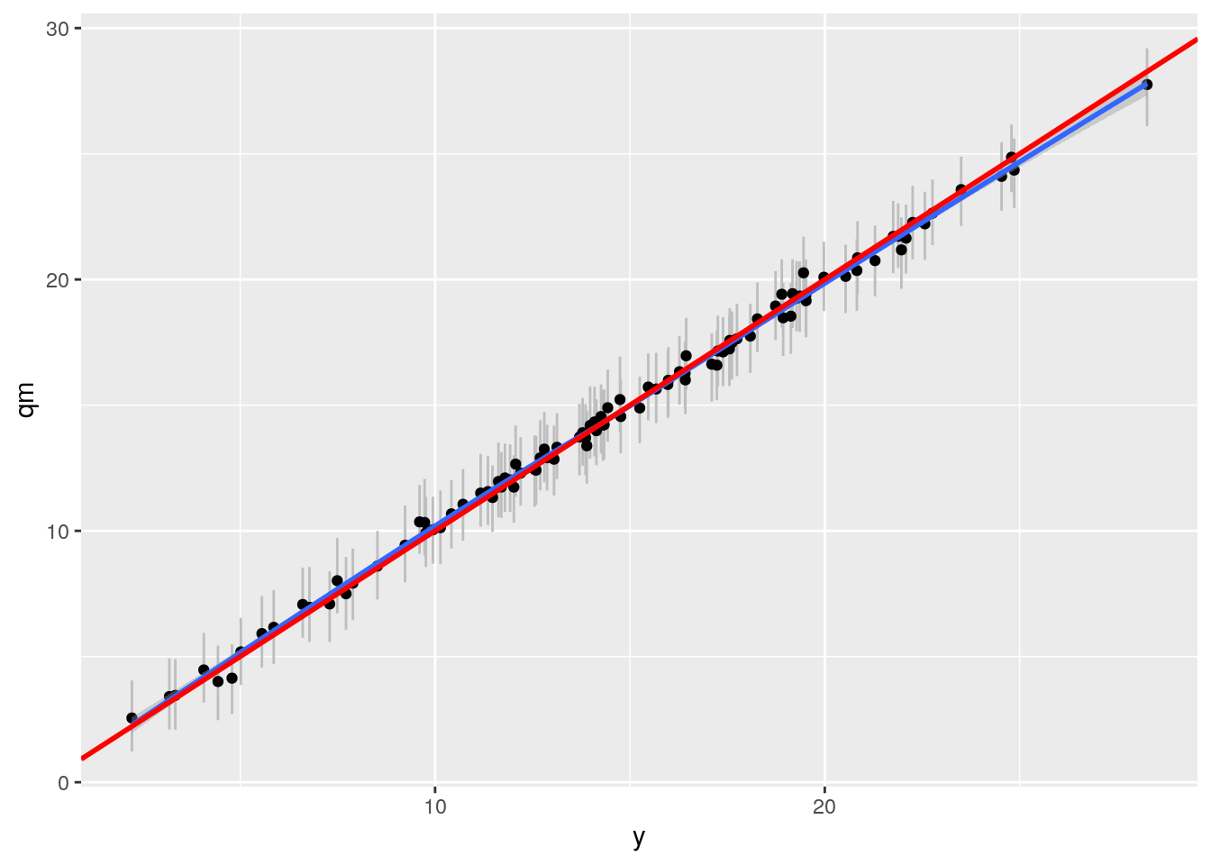
This looks nice.
Fit Grf regression forest on Friedman data
From the manual: Trains a regression forest that can be used to estimate the conditional mean function mu(x) = E[Y | X = x]
if(fullrun){
  reg.forest = regression_forest(x, y, num.trees = 2000)
  saveRDS(reg.forest, "s00.rds")
} else {reg.forest <- readRDS("s00.rds")}
df3 <- CalcPredictionsGRF(x, reg.forest)
df3 <- data.frame(df3, y)
ggplot(df3, aes(x= y, y = qm)) + geom_linerange(aes(ymin = ql, ymax = qu), col = "grey") +
geom_point() +
geom_abline(intercept = 0, slope = 1, col = "red", size = 1)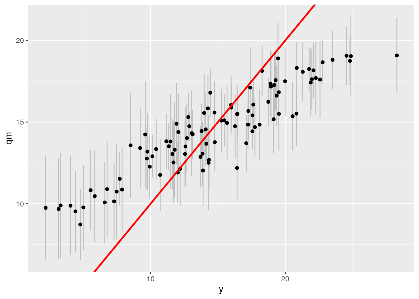
This is pretty bad compared to BART. What's wrong here?
From reference.md: GRF isn't working well on a small dataset
If you observe poor performance on a dataset with a small number of examples, it may be worth trying out two changes:
- Disabling honesty. As noted in the section on honesty above, when honesty is enabled, the training subsample is further split in half before performing splitting. This may not leave enough information for the algorithm to determine high-quality splits.
- Skipping the variance estimate computation, by setting ci.group.size to 1 during training, then increasing sample.fraction. Because of how variance estimation is implemented, sample.fraction cannot be greater than 0.5 when it is enabled. If variance estimates are not needed, it may help to disable this computation and use a larger subsample size for training.
Dataset is pretty small (n=100). Maybe turn of honesty? We cannot turn off variance estimate computation, because we want the CI's
if(fullrun){
  reg.forest2 = regression_forest(x, y, num.trees = 2000,
                                 honesty = FALSE)
  saveRDS(reg.forest2, "s001.rds")
} else {reg.forest2 <- readRDS("s001.rds")}
df2 <- CalcPredictionsGRF(x, reg.forest2)
df2 <- data.frame(df2, y)
grfp <- ggplot(df2, aes(x= y, y = qm)) + geom_linerange(aes(ymin = ql, ymax = qu), col = "grey") +
geom_point() + geom_smooth() +
geom_abline(intercept = 0, slope = 1, col = "red", size = 1)
grfp## `geom_smooth()` using method = 'loess' and formula 'y ~ x'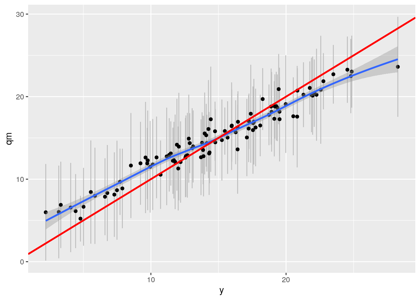
Ah! better now. But Grf still worse than BART. We ran with 2000 trees and turned of honesty. Perhaps dataset too small? Maybe check out the sample.fraction parameter? Sample.fraction is set by default at 0.5, so only half of data is used to grow tree. OR use tune.parameters = TRUE
Compare methods
gp <- plot_grid(bartp, grfp)## `geom_smooth()` using method = 'loess' and formula 'y ~ x'
## `geom_smooth()` using method = 'loess' and formula 'y ~ x'gp 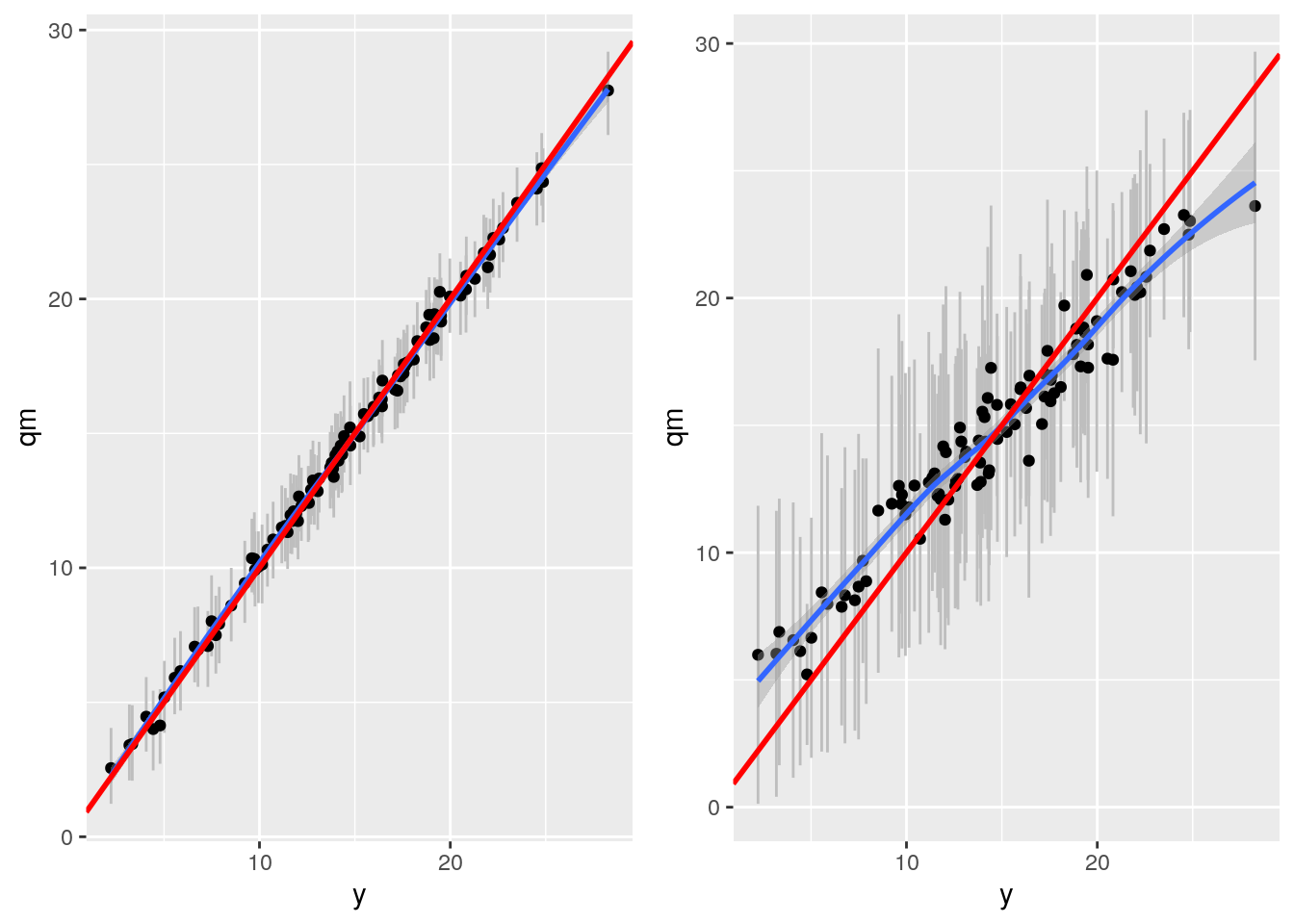
Dataset 2: Simulated data from ACIC 2017
This is a bigger dataset, N=4302.
- Treatment effect \(\tau\) is a function of covariates x3, x24, x14, x15
- Probability of treatment \(\pi\) is a function of covariates x1, x43, x10.
- Outcome is a function of x43
- Noise is a function of x21
head(input_2017[, c(3,24,14,15)])## x_3 x_24 x_14 x_15
## 1 20 white 0 2
## 2 0 black 0 0
## 3 0 white 0 1
## 4 10 white 0 0
## 5 0 black 0 0
## 6 1 white 0 0Check transformed covariates used to create simulated datasets.
# zit hidden in package
head(aciccomp2017:::transformedData_2017)
## x_1 x_3 x_10 x_14 x_15 x_21 x_24 x_43
## 2665 -1.18689448 gt_0 leq_0 leq_0 gt_0 J E -1.0897971
## 22 -0.04543705 leq_0 leq_0 leq_0 leq_0 J B 1.1223750
## 2416 0.13675482 leq_0 leq_0 leq_0 gt_0 J E 0.6136700
## 1350 -0.24062700 gt_0 leq_0 leq_0 leq_0 J E -0.2995632
## 3850 1.02054653 leq_0 leq_0 leq_0 leq_0 I B 0.6136700
## 4167 -1.18689448 gt_0 leq_0 leq_0 leq_0 K E -1.5961206So we find that we should not take the functions in Dorie 2018 (debrief.pdf) literately. x_3 used to calculate the treatment effect is derived from x_3 in the input data. x_24 used to calculate the treatment effect is derived from x_24 in the input data. Both have become binary variables.
Turns out that this was a feature of the 2016 ACIC and IS mentioned in the debrief.pdf
We pick the iid, strong signal, low noise, low confounding first. Actually from estimated PS (W.hat) it seems that every obs has probability of treatment 50%.
parameters_2017[21,]## errors magnitude noise confounding
## 21 iid 1 0 0# easiest?Grab the first replicate.
sim <- dgp_2017(21, 1)Fit BART to ACIC 2017 dataset
Need also counterfactual predictions. Most efficient seems to create x.test with Z reversed. This will give use a y.test as well as y.train in the output. We expect draws for both. Plotting a histogram of the difference gives us the treatment effect with uncertainty.
From the MCMC draws for sigma we infer that we need to drop more "burn in" samples.
Prepare data for BART, including x.test with treatment reversed:
# combine x and y
y <- sim$y
x <- model.matrix(~. ,cbind(z = sim$z, input_2017))

# flip z for counterfactual predictions (needed for BART)
x.test <- model.matrix(~. ,cbind(z = 1 - sim$z, input_2017))
## run BART
#fullrun <- 0
if(fullrun){
set.seed(99)
bartFit <- bart(x, y, x.test, nskip = 350, ntree = 1000)
saveRDS(bartFit, "s2.rds")
} else { bartFit <- readRDS("s2.rds")}
plot(bartFit)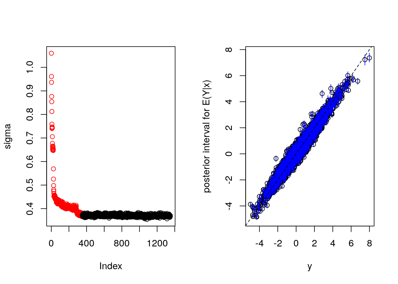
Extract individual treatment effect (ITE / CATE) plus uncertainty from bartfit
This means switching z from 0 to 1 and looking at difference in y + uncertainty in y.
#source("calcPosteriors.R")
sim <- CalcPosteriorsBART(sim, bartFit, "z")

sim <- sim %>% arrange(alpha)

bartp <- ggplot(sim, aes(x = 1:nrow(sim), qm))  +
  geom_linerange(aes(ymin = ql, ymax = qu), col = "grey") +
  geom_point() +
  geom_smooth() + geom_point(aes(y = alpha), col = "red") + ylim(-2.5, 4.5)

bartp
## `geom_smooth()` using method = 'gam' and formula 'y ~ s(x, bs = "cs")'## Warning: Removed 1 rows containing missing values (geom_smooth).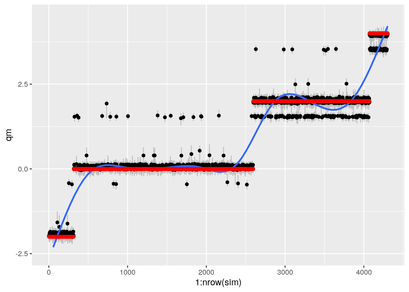
This looks sort of ok, but still weird. Some points it gets REALLY wrong.
Calculate coverage
sim <- sim %>% mutate(in_ci = ql < alpha & qu > alpha)

mean(sim$in_ci)
## [1] 0.4363087Pretty bad coverage. Look into whats going on here. Here it should be 0.9
The iid plot for method 2 gives coverage 0.7 (where it should be 0.95)
Calculate RMSE of CATE
sqrt(mean((sim$alpha - sim$ite)^2))## [1] 0.1587338For All i.i.d. (averaged over 250 replicates averaged over 8 scenarios) method 2 (BART should have RMSE of CATE of 0.35-0.4)
Fit grf to ACIC 2017 dataset
need large num.trees for CI.
# prep data for Grf
# combine x and y
sim <- dgp_2017(21, 1)

Y <- sim$y
X <- model.matrix(~. ,input_2017)
W = sim$z

# Train a causal forest.
#fullrun <- 0

if(fullrun){
  grf.fit_alt <- causal_forest(X, Y, W, num.trees = 500)
  saveRDS(grf.fit_alt, "s3.rds")
} else{grf.fit_alt <- readRDS("s3.rds")}
It appears that using 4000 trees consumes too much memory (bad_alloc)
Compare predictions vs true value
df_sep2 <- CalcPredictionsGRF(X, grf.fit_alt)

df_sep2 <- data.frame(df_sep2, Y, W, TAU = sim$alpha)

df_sep2 <- df_sep2 %>% arrange(TAU)

grfp <- ggplot(df_sep2, aes(x = 1:nrow(df_sep2), y = qm))   +
  geom_linerange(aes(ymin = ql, ymax = qu), col = "grey") + geom_point() + geom_smooth() +
  geom_point(aes(y = TAU), col = "red") + ylim(-2.5, 4.5)

grfp
## `geom_smooth()` using method = 'gam' and formula 'y ~ s(x, bs = "cs")'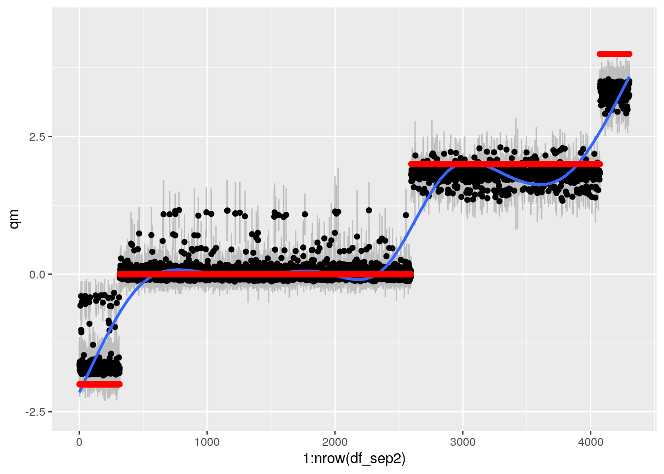
This works ok now.
Compare both methods
gp <- plot_grid(bartp, grfp)## `geom_smooth()` using method = 'gam' and formula 'y ~ s(x, bs = "cs")'## Warning: Removed 1 rows containing missing values (geom_smooth).## `geom_smooth()` using method = 'gam' and formula 'y ~ s(x, bs = "cs")'gp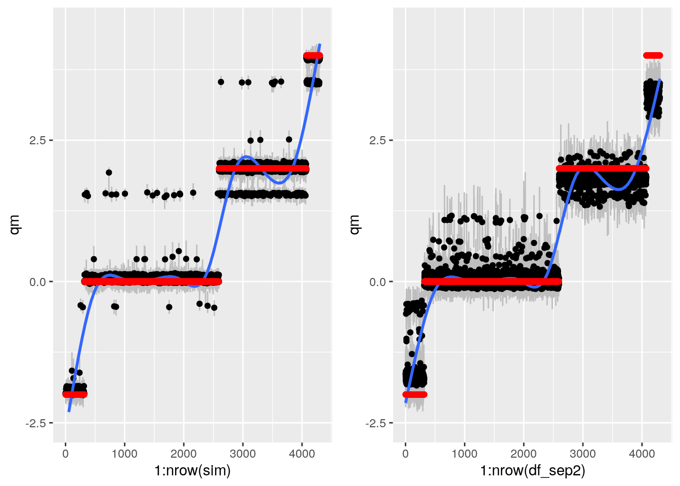
Dataset 3: simulated data used by grf example
THis dataset is used in the Grf manual page. Size N = 2000. Probability of treatment function of X1. Treatment effect function of X1.
# Generate data.
set.seed(123)
n = 2000; p = 10
X = matrix(rnorm(n*p), n, p)

# treatment
W = rbinom(n, 1, 0.4 + 0.2 * (X[,1] > 0))
# outcome (parallel max)
Y = pmax(X[,1], 0) * W + X[,2] + pmin(X[,3], 0) + rnorm(n)

# TAU is true treatment effect
df <- data.frame(X, W, Y, TAU = pmax(X[,1], 0))
Fit GRF
Default settings are honesty = TRUE.
# Train a causal forest.
if(fullrun){
  tau.forest = causal_forest(X, Y, W, num.trees = 2000)
  saveRDS(tau.forest, "s4.rds")
} else {tau.forest <- readRDS("s4.rds")}
OOB predictions
From the GRF manual:
Given a test example, the GRF algorithm computes a prediction as follows:
For each tree, the test example is 'pushed down' to determine what leaf it falls in.
Given this information, we create a list of neighboring training examples, weighted by how many times the example fell in the same leaf as the test example.
A prediction is made using this weighted list of neighbors, using the relevant approach for the type of forest. In causal prediction, we calculate the treatment effect using the outcomes and treatment status of the neighbor examples.
Those familiar with classic random forests might note that this approach differs from the way forest prediction is usually described. The traditional view is that to predict for a test example, each tree makes a prediction on that example. To make a final prediction, the tree predictions are combined in some way, for example through averaging or through 'majority voting'. It's worth noting that for regression forests, the GRF algorithm described above is identical this 'ensemble' approach, where each tree predicts by averaging the outcomes in each leaf, and predictions are combined through a weighted average.
# Estimate treatment effects for the training data using out-of-bag prediction.
tau.hat.oob = predict(tau.forest)

res <- data.frame(df, pred = tau.hat.oob$predictions)

ggplot(res, aes(x = X1, y = pred)) + geom_point() + geom_smooth() + geom_abline(intercept = 0, slope = 1) +
  geom_line(aes(y = TAU), col = "red", size = 1)
## `geom_smooth()` using method = 'gam' and formula 'y ~ s(x, bs = "cs")'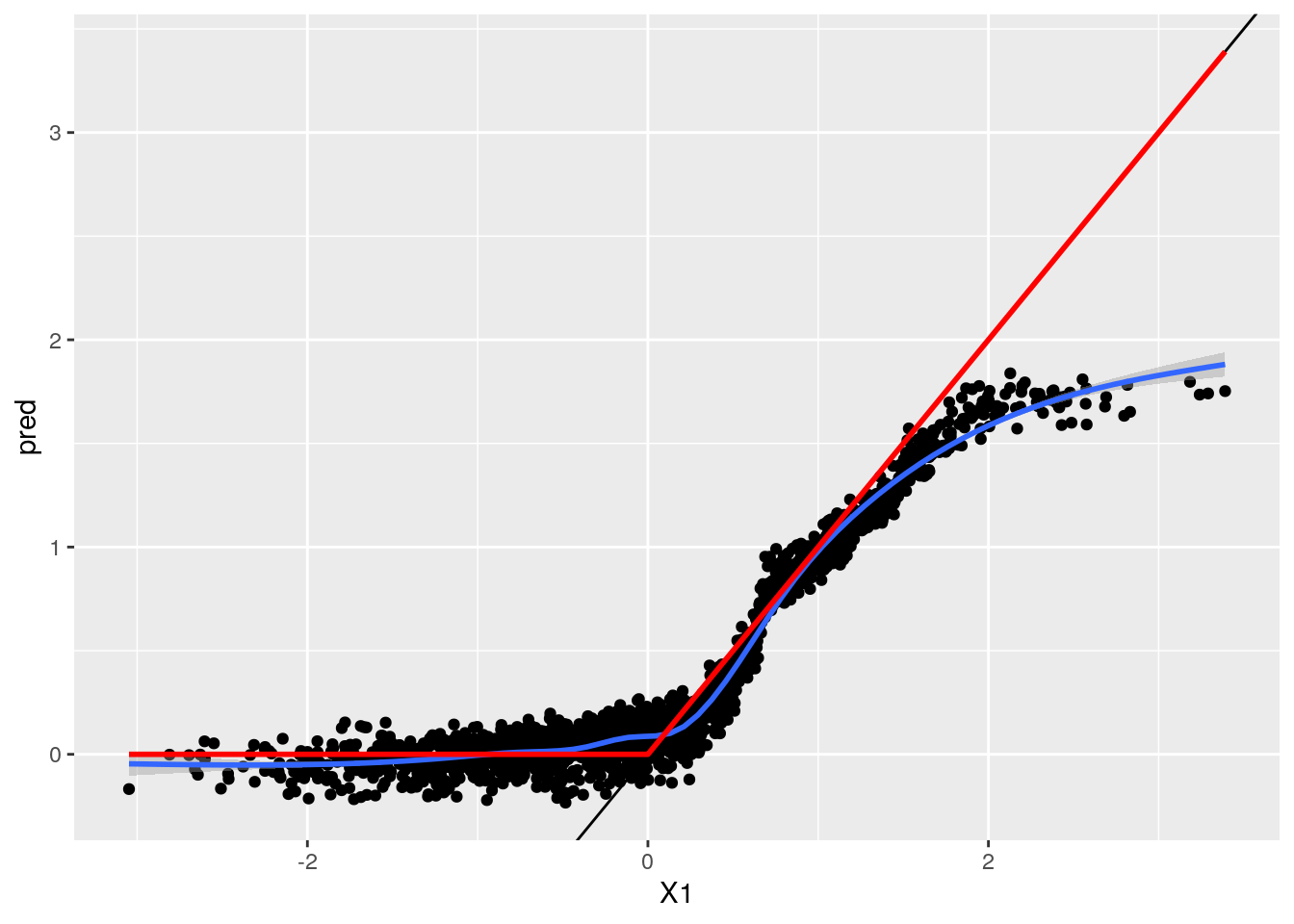
ATE & ATT
# Estimate the conditional average treatment effect on the full sample (CATE).
average_treatment_effect(tau.forest, target.sample = "all")
## estimate std.err
## 0.37316437 0.04795009mean(res$TAU)## [1] 0.4138061# Estimate the conditional average treatment effect on the treated sample (CATT).
# Here, we don't expect much difference between the CATE and the CATT, since
# treatment assignment was randomized.
average_treatment_effect(tau.forest, target.sample = "treated")## estimate std.err
## 0.47051526 0.04850751mean(res[res$W == 1,]$TAU)## [1] 0.5010723Fit more trees for CI's
# Add confidence intervals for heterogeneous treatment effects; growing more
# trees is now recommended.
if(fullrun){
  tau.forest_big = causal_forest(X, Y, W, num.trees = 4000)
  saveRDS(tau.forest_big, "s5.rds")
} else {tau.forest_big <- readRDS("s5.rds")}
Plot CI's
## PM
#source("CalcPosteriors.R")
df_res <- CalcPredictionsGRF(df, tau.forest_big)

grfp <- ggplot(df_res, aes(x = X1, y = qm)) +
  geom_linerange(aes(ymin = ql, ymax = qu), col = "grey") +
  geom_point()  +
  geom_smooth() + geom_line(aes(y = TAU), col = "red", size = 1) +
   ylim(-1,3.5)

grfp
## `geom_smooth()` using method = 'gam' and formula 'y ~ s(x, bs = "cs")'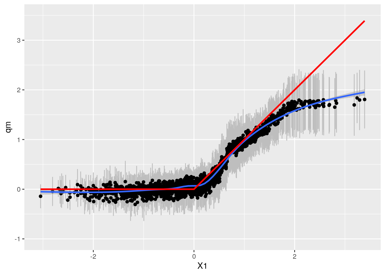
Fit BART on this dataset
x.train <- model.matrix(~. ,data.frame(W, X))
x.test <- model.matrix(~. ,data.frame(W = 1 - W, X))
y.train <- Y

if(fullrun){
  bartFit <- bart(x.train, y.train, x.test, ntree = 2000, ndpost = 1000, nskip = 100)
  saveRDS(bartFit, "s10.rds")
} else {bartFit <- readRDS("s10.rds")}
plot(bartFit)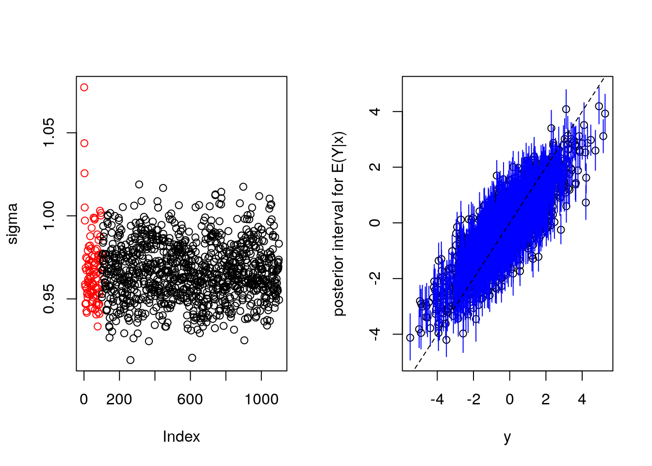
BART: Check fit and CI's
#source("calcPosteriors.R")
sim <- CalcPosteriorsBART(df, bartFit, treatname = "W")


bartp <- ggplot(sim, aes(x = X1, qm)) + geom_linerange(aes(ymin = ql, ymax = qu), col = "grey") +
  geom_point() + geom_smooth() +
  geom_line(aes(y = TAU), col = "red", size = 1) + ylim(-1,3.5)

bartp
## `geom_smooth()` using method = 'gam' and formula 'y ~ s(x, bs = "cs")'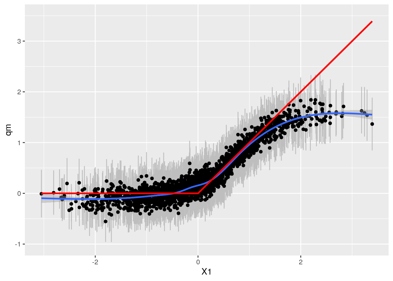
Compare
gp <- plot_grid(bartp, grfp)## `geom_smooth()` using method = 'gam' and formula 'y ~ s(x, bs = "cs")'
## `geom_smooth()` using method = 'gam' and formula 'y ~ s(x, bs = "cs")'gp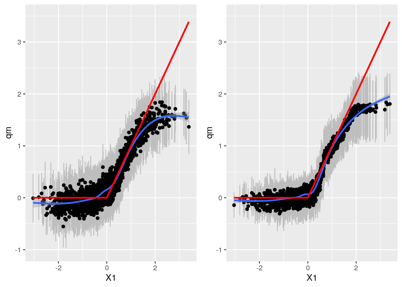
Here Grf appears more accurate. Mental note: Both W and TAU function of X1.
Dataset 4: Fit separate grf forests for Y and W
This dataset has a complex propensity of treatment function (Exponential of X1 and X2), as well as hetergeneous treatment effect that is exponential function of X3. It has size N=4000.
# In some examples, pre-fitting models for Y and W separately may
# be helpful (e.g., if different models use different covariates).
# In some applications, one may even want to get Y.hat and W.hat
# using a completely different method (e.g., boosting).
set.seed(123)
# Generate new data.
n = 4000; p = 20
X = matrix(rnorm(n * p), n, p)
TAU = 1 / (1 + exp(-X[, 3]))
W = rbinom(n ,1, 1 / (1 + exp(-X[, 1] - X[, 2])))
Y = pmax(X[, 2] + X[, 3], 0) + rowMeans(X[, 4:6]) / 2 + W * TAU + rnorm(n)

df_sep4 <- data.frame(X, TAU, W, Y)
Grf two-step: First fit model for W (PS)
Regression forest to predict W from X. This is a propensity score.
if(fullrun){
  forest.W <- regression_forest(X, W, tune.parameters = c("min.node.size", "honesty.prune.leaves"),
                               num.trees = 2000)
  saveRDS(forest.W, "s6.rds")
} else {forest.W <- readRDS("s6.rds")}

W.hat = predict(forest.W)$predictions
Grf:Then Fit model for Y, selecting covariates
This predict Y from X, ignoring treatment.
if(fullrun){
  forest.Y = regression_forest(X, Y, tune.parameters = c("min.node.size", "honesty.prune.leaves"),
                               num.trees = 2000)
  saveRDS(forest.Y, "s7.rds")
} else {forest.Y <- readRDS("s7.rds")}

Y.hat = predict(forest.Y)$predictions
Grf:Select variables that predict Y.
forest.Y.varimp = variable_importance(forest.Y)
# Note: Forests may have a hard time when trained on very few variables
# (e.g., ncol(X) = 1, 2, or 3). We recommend not being too aggressive
# in selection.
selected.vars = which(forest.Y.varimp / mean(forest.Y.varimp) > 0.2)
This selects five variables of 20. Indeed these are the variables that were used to simulate Y.
Grf: Finally, Fit causal forest using PS and selected covariates
if(fullrun){
tau.forest2 = causal_forest(X[, selected.vars], Y, W,
                           W.hat = W.hat, Y.hat = Y.hat,
                           tune.parameters = c("min.node.size", "honesty.prune.leaves"),
                           num.trees = 4000)
  saveRDS(tau.forest2, "s8.rds")
} else {tau.forest2 <- readRDS("s8.rds")}
Grf: Check fit and CI's
df_sep2 <- CalcPredictionsGRF(df_sep4[,selected.vars], tau.forest2)

grfp <- ggplot(df_sep2, aes(x = X3, y = qm))   +
  geom_linerange(aes(ymin = ql, ymax = qu), col = "grey") + geom_point() +
  geom_smooth() +
  geom_line(aes(y = TAU), col = "red", size = 1) + ylim(-0.7,2)

grfp
## `geom_smooth()` using method = 'gam' and formula 'y ~ s(x, bs = "cs")'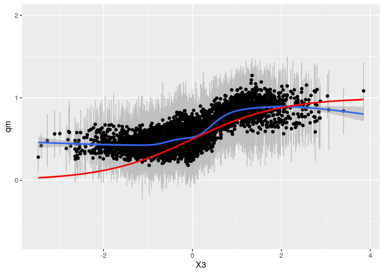 This looks ok.
Fit BART on this dataset
x.train <- model.matrix(~. ,data.frame(W, X))
x.test <- model.matrix(~. ,data.frame(W = 1 - W, X))
y.train <- Y

if(fullrun){
  bartFit <- bart(x.train, y.train, x.test, ntree = 4000)
  saveRDS(bartFit, "s9.rds")
} else {bartFit <- readRDS("s9.rds")}
plot(bartFit)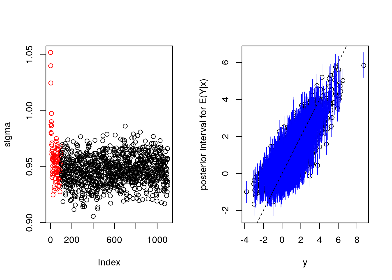
BART: Check fit and CI's
#source("calcPosteriors.R")
sim <- CalcPosteriorsBART(df_sep4, bartFit, treatname = "W")


bartp <- ggplot(sim, aes(x = X3, qm)) + geom_linerange(aes(ymin = ql, ymax = qu), col = "grey") +
  geom_point() + geom_smooth() +
  geom_line(aes(y = TAU), col = "red", size = 1) + ylim(-0.7,2)

bartp
## `geom_smooth()` using method = 'gam' and formula 'y ~ s(x, bs = "cs")'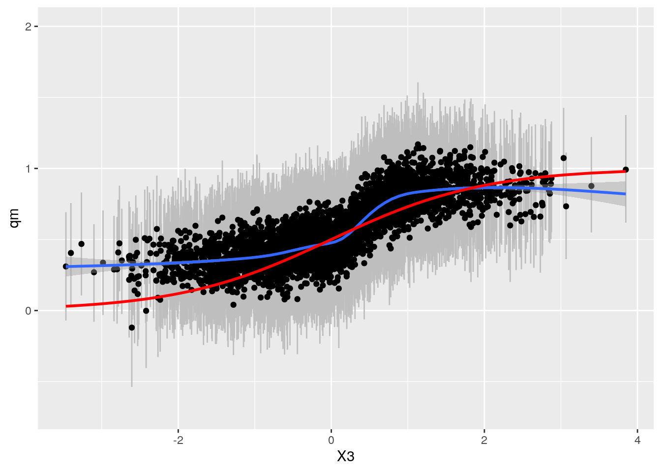
Compare BART and grf
gp <- plot_grid(bartp, grfp)## `geom_smooth()` using method = 'gam' and formula 'y ~ s(x, bs = "cs")'
## `geom_smooth()` using method = 'gam' and formula 'y ~ s(x, bs = "cs")'gp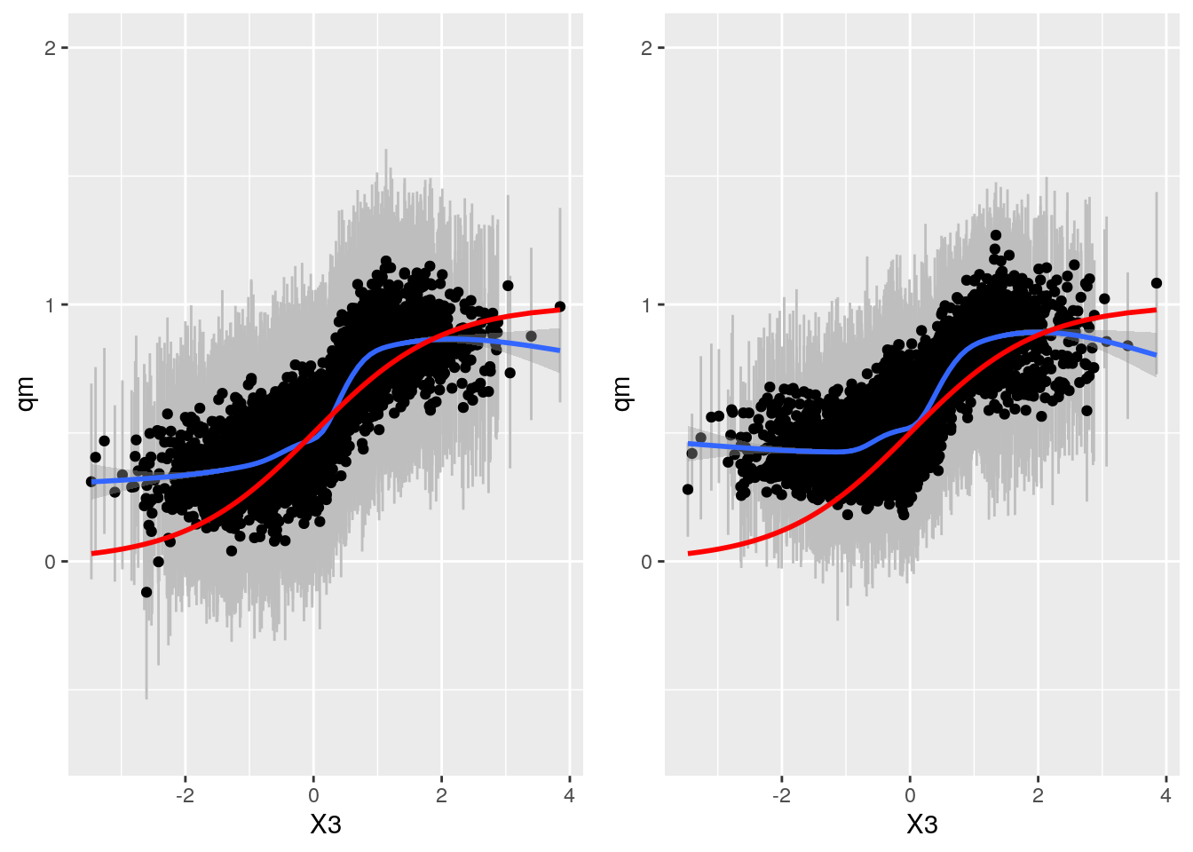
Very similar results. BART appears slightly more accurate, especially for low values of X3.
Gertjan Verhoeven
Data Scientist / Policy Advisor
Gertjan Verhoeven is a research scientist currently at the Dutch Healthcare Authority, working on health policy and statistical methods. Follow me on Twitter or Mastodon to receive updates on new blog posts. Statistics posts using R are featured on R-Bloggers.