
OpenAI Gym's FrozenLake: Converging on the true Q-values
(Photo by Ryan Fishel on Unsplash)
This blog post concerns a famous “toy” problem in Reinforcement Learning, the FrozenLake environment. We compare solving an environment with RL by reaching maximum performance versus obtaining the true state-action values \(Q_{s,a}\). In doing so I learned a lot about RL as well as about Python (such as the existence of a ggplot clone for Python, plotnine, see this blog post for some cool examples).
FrozenLake was created by OpenAI in 2016 as part of their Gym python package for Reinforcement Learning. Nowadays, the interwebs is full of tutorials how to “solve” FrozenLake. Most of them focus on performance in terms of episodic reward. As soon as this maxes out the algorithm is often said to have converged. For example, in this question on Cross-Validated about Convergence and Q-learning:
In practice, a reinforcement learning algorithm is considered to converge when the learning curve gets flat and no longer increases.
Now, for Q-learning it has been proven that, under certain conditions, the Q-values convergence to their true values. But does this happens when the performance maxes out? In this blog we’ll see that this is not generally the case.
We start with obtaining the true, exact state-action values. For this we use Dynamic Programming (DP). Having implemented Dynamic Programming (DP) for the FrozenLake environment as an exercise notebook already (created by Udacity, go check them out), this was a convenient starting point.
Loading the packages and modules
We need various Python packages and modules.
# data science packages
import numpy as np
import pandas as pd
import plotnine as p9
import matplotlib.pyplot as plt
%matplotlib inline

# RL algorithms
from qlearning import *
from dp import *

# utils
from helpers import *
from plot_utils import plot_values
import copy
import dill

from frozenlake import FrozenLakeEnv

env = FrozenLakeEnv(is_slippery = True)
Frozen Lake Environment description
Winter is here. You and your friends were tossing around a frisbee at the park when you made a wild throw that left the frisbee out in the middle of the lake (G). The water is mostly frozen (F), but there are a few holes (H) where the ice has melted.
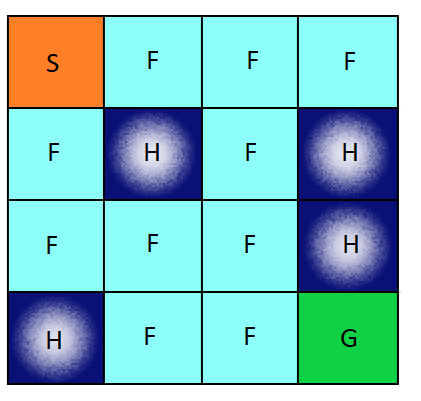
If you step into one of those holes, you’ll fall into the freezing water. At this time, there’s an international frisbee shortage, so it’s absolutely imperative that you navigate across the lake and retrieve the disc. However, the ice is slippery, so you won’t always move in the direction you intend.
The episode ends when you reach the goal or fall in a hole. You receive a reward of 1 if you reach the goal, and zero otherwise.
The agent moves through a \(4 \times 4\) gridworld, with states numbered as follows:
[[ 0  1  2  3]
 [ 4  5  6  7]
 [ 8  9 10 11]
 [12 13 14 15]]
and the agent has 4 potential actions:
LEFT = 0
DOWN = 1
RIGHT = 2
UP = 3
The FrozenLake Gym environment has been amended to make the one-step dynamics accessible to the agent. For example, if we are in State s = 1 and we perform action a = 0, the probabilities of ending up in new states, including the associated rewards are contained in the \(P_{s,a}\) array:
env.P[1][0][(0.3333333333333333, 1, 0.0, False),
(0.3333333333333333, 0, 0.0, False),
(0.3333333333333333, 5, 0.0, True)]The FrozenLake environment is highly stochastic, with a very sparse reward: only when the agent reaches the goal, a reward of +1 is obtained. This means that if we do not set a discount rate, the agent can keep on wandering around without receiving a learning “signal” that can be propagated back through the preceding state-actions (since falling into the holes does not result in a negative reward) and thus learning very slowly. We will focus on the discounting case (gamma = 0.95) for this reason (less computation needed for convergence), but compare also with the undiscounted case.
Solving Frozen Lake using DP
Let us solve FrozenLake first for the no discounting case (gamma = 1).
The Q-value for the first state will then tell us the average episodic reward, which for FrozenLake translates into the percentage of episodes in which the Agent succesfully reaches its goal.
policy_pi, V_pi = policy_iteration(env, gamma = 1, theta=1e-9, \
                                   verbose = False)


plot_values(V_pi)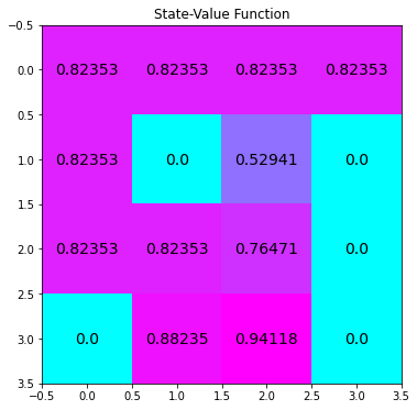
The Q-value for state s = 0 is 0.824. This means that for gamma = 1 and following an optimal policy \(\pi^*\), 82.4% of all episodes ends in succes.
As already mentioned above, for computational reasons we will apply Q-learning to the environment with gamma = 0.95. So… lets solve FrozenLake for gamma = 0.95 as well:
# obtain the optimal policy and optimal state-value function
policy_pi_dc, V_pi_dc = policy_iteration(env, gamma = 0.95, theta=1e-9, \
                                   verbose = False)

Q_perfect = create_q_dict_from_v(env, V_pi_dc, gamma = 0.95)

df_true = convert_vals_to_pd(V_pi_dc)

plot_values(V_pi_dc)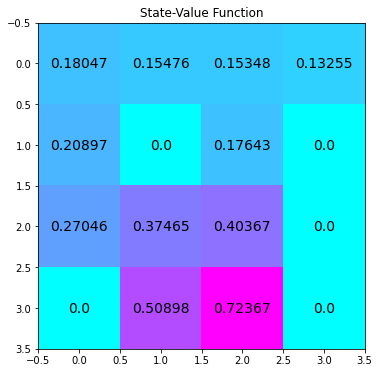
Now, comparing the optimal policies for gamma = 0.95 and for gamma = 1 (not shown here) we find that they are not the same. Therefore, 82.4% succes rate is likely an upper bound for gamma = 0.95, since introducing discounting in this stochastic environment can (intuitively) either have no effect on the optimal policy, or favor more risky (lower succes rate) but faster (less discounting) policies, leading to a lower overall succes rate.
For example, for the undiscounted case, the Agent is indifferent in choosing direction in the first state. If it ends up going right , it can choose UP and wander around at the top row at no cost until it reaches the starting state again. As soon as this wandering around gets a cost by discounting we see (not shown) that the Agent is no longer indifferent, and does NOT want to end up wandering in the top row, but chooses to play LEFT in state s = 0 instead.
Checking the performance of an optimal greedy policy based on perfect Q-values
Now that we have the \(Q_{s,a}\) values corresponding to the optimal policy given that gamma = 0.95, we can check its performance. To do so, we use brute force and simulate the average reward under the optimal policy for a large number of episodes.
To do so, I wrote a function test_performance() by taking the q_learning() function, removing the learning (Q-updating) part and setting epsilon to zero when selecting an action (i.e. a pure greedy policy based on a given Q-table).
Playing around with the binomial density in R (summary(rbinom(1e5, 1e5, prob = 0.8)/1e5) tells me that choosing 100.000 episodes gives a precision of around three decimals in estimating the probability of succes. This is good enough for me.
# Obtain Q for Gamma = 0.95 and convert to defaultdict
Q_perfect = create_q_dict_from_v(env, V_pi_dc, gamma = 0.95)

fullrun = 0

if fullrun == 1:
    d = []
    runs = 100
    for i in range(runs):
        avg_scores = test_performance(Q_perfect, env, num_episodes = 1000, \
                                   plot_every = 1000, verbose = False)
        d.append({'run': i,
                 'avg_score': np.mean(avg_scores)})
        print("\ri {}/{}".format(i, runs), end="")
        sys.stdout.flush()

    d_perfect = pd.DataFrame(d)
    d_perfect.to_pickle('cached/scores_perfect_0.95.pkl')
else:
    d_perfect = pd.read_pickle('cached/scores_perfect_0.95.pkl')
round(np.mean(d_perfect.avg_score), 3)0.781Thus, we find that with the true optimal policy for gamma = 0.95, in the long run 78% of all episodes is succesful. This is therefore the expected plateau value for the learning curve in Q-learning, provided that the exploration rate has become sufficiently small.
Let’s move on to Q-learning and convergence.
“Solving” FrozenLake using Q-learning
The typical RL tutorial approach to solve a simple MDP as FrozenLake is to choose a constant learning rate, not too high, not too low, say \(\alpha = 0.1\). Then, the exploration parameter \(\epsilon\) starts at 1 and is gradually reduced to a floor value of say \(\epsilon = 0.0001\).
Lets solve FrozenLake this way, monitoring the learning curve (average reward per episode) as it learns, and compare the learned Q-values with the true Q-values found using DP.
I wrote Python functions that generate a decay schedule, a 1D numpy array of \(\epsilon\) values, with length equal to the total number of episode the Q-learning algorithm is to run. This array is passed on to the Q-learning algorithm, and used during learning.
It is helpful to visualize the decay schedule of \(\epsilon\) to check that it is reasonable before we start to use them with our Q-learning algorithm. I played around with the decay rate until the “elbow” of the curve is around 20% of the number of episodes, and reaches the desired minimal end value (\(\epsilon = 0.0001\)).
def create_epsilon_schedule(num_episodes,  \
                       epsilon_start=1.0, epsilon_decay=.9999, epsilon_min=1e-4):
    x = np.arange(num_episodes)+1
    y = np.full(num_episodes, epsilon_start)
    y = np.maximum((epsilon_decay**x)*epsilon_start, epsilon_min)
    return y

epsilon_schedule = create_epsilon_schedule(100_000)

plot_schedule(epsilon_schedule, ylab = 'Epsilon')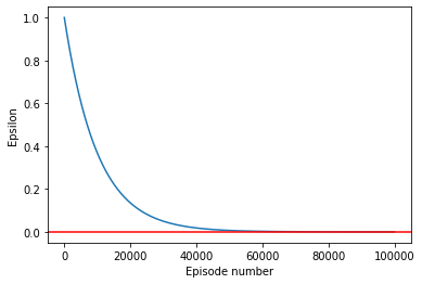
My version of the Q-learning algorithm has slowly evolved to include more and more lists of things to monitor during the execution of the algorithm. Every 100 episodes, a copy of \(Q^{*}_{s}\) and of \(Q_{s, a}\) is stored in a list, as well as the average reward over this episode, as well as the final \(Q_{s,a}\) table, and \(N_{s,a}\) that kept track of how often each state-action was chosen. The dill package is used to store these datastructures on disk to avoid the need to rerun the algorithm every time the notebook is run.
# K / N + K decay learning rate schedule
# fully random policy

plot_every = 100

n_episodes = len(epsilon_schedule)

fullrun = 0

random.seed(123)
np.random.seed(123)

if fullrun == 1:
    Q_sarsamax, N_sarsamax, avg_scores, Qlist, Qtable_list = q_learning(env, num_episodes = n_episodes, \
                                                eps_schedule = epsilon_schedule,\
                                                alpha = 0.1, \
                                                gamma =  0.95, \
                                                plot_every = plot_every, \
                                                verbose = True, log_full = True)

    with open('cached/es1_Q_sarsamax.pkl', 'wb') as f:
        dill.dump(Q_sarsamax, f)
    with open('cached/es1_avg_scores.pkl', 'wb') as f:
        dill.dump(avg_scores, f)
    with open('cached/es1_Qlist.pkl', 'wb') as f:
        dill.dump(Qlist, f)
    with open('cached/es1_Qtable_list.pkl', 'wb') as f:
        dill.dump(Qtable_list, f)
else:
    with open('cached/es1_Q_sarsamax.pkl', 'rb') as f:
        Q_sarsamax = dill.load(f)
    with open('cached/es1_avg_scores.pkl', 'rb') as f:
        avg_scores = dill.load(f)
    with open('cached/es1_Qlist.pkl', 'rb') as f:
        Qlist = dill.load(f)
    with open('cached/es1_Qtable_list.pkl', 'rb') as f:
        Qtable_list = dill.load(f)

Q_es1_lasttable = [np.max(Q_sarsamax[key]) if key in Q_sarsamax \
     else 0 for key in np.arange(env.nS)]
Lets plot the learning curve. Here plotnine, a ggplot clone in Python comes in handy.
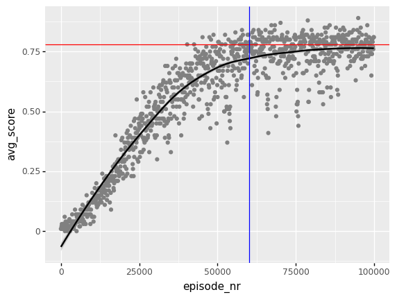
As we can see below, the “recipe” for solving FrozenLake has worked really well. The displayed red line gives the theoretical optimal performance for gamma = 0.95, I used a loess smoother so we can more easily compare the Q-learning results with the theoretical optimum.
We can see that the Q-learning algorithm has indeed found a policy that performs optimal. This appears to happen at around 60.000 episodes. We return to this later.
# plot performance
df_scores = pd.DataFrame(
    {'episode_nr': np.linspace(0,n_episodes,len(avg_scores),endpoint=False),
     'avg_score': np.asarray(avg_scores)})

(p9.ggplot(data = df_scores.loc[df_scores.episode_nr > -1], mapping = p9.aes(x = 'episode_nr', y = 'avg_score'))
    + p9.geom_point(colour = 'gray')
    + p9.geom_smooth(method = 'loess')
    + p9.geom_hline(yintercept = 0.781, colour = "red")
    + p9.geom_vline(xintercept = 60_000, color = "blue"))
But now comes the big question: did the \(Q^{*}_{a}\) estimates converge onto the true values as well?
q_showdown = pd.DataFrame(
    {'Q_es1_lasttable': Q_es1_lasttable,
     'q_true': V_pi_dc})
q_showdown['state'] = range(16)

q_showdown = pd.melt(q_showdown, ['state'])

(p9.ggplot(data = q_showdown, mapping = p9.aes(x = 'state', y = 'value', color = 'factor(variable)'))
+ p9.geom_point(size = 5, shape = 'x'))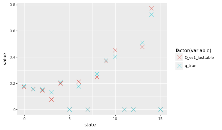
Nope, they did not. Ok, most learned Q-values are close to their true values, but they clearly did not converge exactly to their true value.
Plotting the learning curves for all the state-action values
To really understand what is going on, I found it helpful to plot the learning curves for all the 16 x 4 = 64 state-action values at the same time. Here plotnine really shines. I leave out the actual estimates, and only plot a loess smoothed curve for each of the state-action values over time.
# convert to pandas df
dfm = list_of_tables_to_df(Qtable_list)
#10 s
(p9.ggplot(data = dfm.loc[(dfm.episode > -1)], mapping = p9.aes(x = 'episode', y = 'value', group = 'action', color = 'factor(action)'))
#+ p9.geom_point(shape = 'x')
+ p9.geom_smooth(method = 'loess')
+ p9.geom_hline(data = df_true, mapping = p9.aes(yintercept = 'value'), color = 'red')
+ p9.geom_vline(xintercept = 600, color = 'blue')
+ p9.facet_wrap("variable", ncol = 4)
+ p9.theme(subplots_adjust={'wspace':0.4}) # fix a displaying issue
)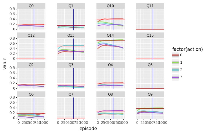
First the main question: what about convergence of \(Q^{*}_{a}\)? For this we need only to look, for each state, at the action with the highest value, and compare that to the true value (red horizontal lines). Most of the values appear to have converged to a value close to the true value, but Q3 is clearly still way off. Note that we using smoothing here to average out the fluctuations around the true value.
We noted earlier that at around episode 60.000, the optimal policy emerges and the learning curve becomes flat. Now, the most obvious reason why performance increases is because the value of \(\epsilon\) is decaying, so the deleterious effects of exploration should go down, and performance should go up.
Another reason that performance goes up could be that the greedy policy is improving. It is interesting to examine whether at this point, meaningfull changes in the greedy policy still occur. Meaningfull changes in policy are caused by changes in the estimated state-action values. For example, we might expect two or more state-action value lines crossing, with the “right” action becoming dominant over the “wrong” action. Is this indeed the case?
Indeed, from the plot above, with the change point at around episode 600 (x 100),a change occurs in Q6, where the actions 0 and 2 cross. However, from the true Q-value table (not shown) we see that both actions are equally rewarding, so the crossing has no effect on performance. Note that only one of the two converges to the true value, because the exploration rate becomes so low that learning for the other action almost completely stops in the end.
lets zoom in then at the states that have low expected reward, Q0, Q1, Q2, and Q3. These are difficult to examine in the plot above, and have actions with expected rewards that are similar and therefore more difficult to resolve (BUT: since the difference in expected reward is small, the effect of resolving them on the overall performance is small as well). For these we plot the actual state-actions values:
(p9.ggplot(data = dfm[dfm.variable.isin(['Q0', 'Q1','Q2', 'Q3'])], mapping = p9.aes(x = 'episode', y = 'value', group = 'action', color = 'factor(action)'))
    + p9.geom_point(shape = 'x')
    #+ p9.geom_smooth(method = 'loess')
    + p9.geom_hline(data = df_true[df_true.variable.isin(['Q0', 'Q1','Q2', 'Q3'])], mapping = p9.aes(yintercept = 'value'), color = 'red')
    + p9.geom_vline(xintercept = 600, color = 'blue')
    + p9.facet_wrap("variable", scales = 'free_y')
    + p9.theme(subplots_adjust={'wspace':0.15})
)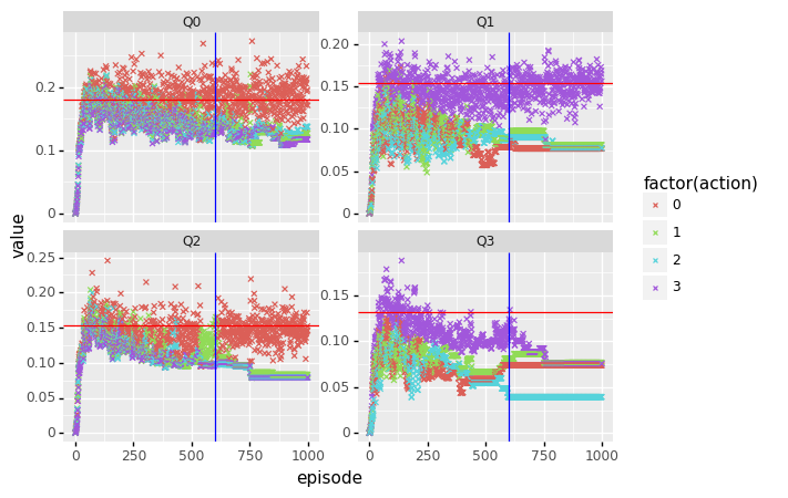
From Q1, Q2 and Q3, we can see that exploration really goes down at around episode 500 (x 100) (\(\epsilon\) at this point is 0.007), and with the optimal action standing out already long before reaching this point.
Only with Q2 there is a portion of the learning curve where action 1 has the highest value, and is chosen for quite some time before switching back to action 0 again at around episode 60.000. Let’s compare with the true values for Q2:
Q_perfect[2]array([0.15347714, 0.14684971, 0.14644451, 0.13958106])Indeed, the difference in expected reward between the actions in state 2 is really small, and because of the increasingly greedy action selection, only action 0 converges to its true values, with the other values “frozen” in place because of the low exploration rate.
Now, after analyzing what happens if we apply the “cookbook” approach to solving problems using RL, let’s change our attention to getting convergence for preferably ALL the state-action values.
Q-learning: Theoretical sufficient conditions for convergence
According to our RL bible (Sutton & Barto), to obtain exact convergence, we need two conditions to hold.
- The first is that all states continue to be visited, and
- the second is that the learning rate goes to zero.
Continuous exploration: visiting all the states
The nice thing of Q-learning is that it is an off-policy learning algorithm. This means that no matter what the actual policy is used to explore the states, the Q-values we learn correspond to the expected reward when following the optimal policy. Which is quite miraculous if you ask me.
Now, our (admittedly, a bit academic) goal is getting all of the learned state values as close as possible to the true values. An epsilon-greedy policy with a low \(epsilon\) would spent a lot of time by choosing state-actions that are on the optimal path between start and goal state, and would only rarely visit low value states, or choose low value state-actions.
Because we can choose any policy we like, I chose a completely random policy. This way, the Agent is more likely to end up in low value states and estimate the Q-values of those state-actions accurately as well.
Note that since theFrozen Lake enviroment has a lot of inherent randomness already because of the ice being slippery, a policy with a low \(\epsilon\) (most of the time exploiting and only rarely exploring) will still bring the agent in low values states, but this would require much more episodes.
Convergence and learning rate schedules
For a particular constant learning rate, provided that it is not too high, the estimated Q-values will converge to a situation where they start to fluctuate around their true values. If we subsequently lower the learning rate, the scale of the fluctuations (their variance) will decrease. If the learning rate is gradually decayed to zero, the estimates will converge. According to Sutton & Barto (2018), the decay schedule of \(\alpha\) must obey two constraints to assure convergence: (p 33).
- sum of increments must go to infinity
- sum of the square of increments must go to zero
On the interwebs, I found two formulas that are often used to decay hyperparameters of Reinforcement Learning algorithms:
\(\alpha_n = K / (K + n)\) (Eq. 1)
\(\alpha_n = \Sigma^{\infty}_{n = 1} \delta^n \alpha_0\) (Eq. 2)
Again, just as with the decay schedule for \(\epsilon\), it is helpful to visualize the decay schedules to check that they are reasonable before we start to use them with our Q-learning algorithm.
# Eq 1
def create_alpha_schedule(num_episodes, \
                     alpha_K = 100, alpha_min = 1e-3):
    x = np.arange(num_episodes)+1
    y = np.maximum(alpha_K/(x + alpha_K), alpha_min)
    return y

# Eq 2
def create_alpha_schedule2(num_episodes,  \
                       alpha_start=1.0, alpha_decay=.999, alpha_min=1e-3):
    x = np.arange(num_episodes)+1
    y = np.full(num_episodes, alpha_start)
    y = np.maximum((alpha_decay**x)*alpha_start, alpha_min)
    return y
I played a bit with the shape parameter to get a curve with the “elbow” around 20% of the episodes.
alpha_schedule = create_alpha_schedule(num_episodes = 500_000, \
                                       alpha_K = 5_000)

plot_schedule(alpha_schedule, ylab = 'Alpha')
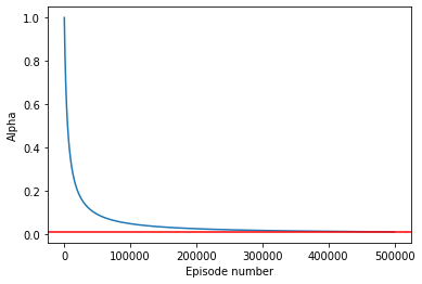
round(min(alpha_schedule), 3)0.01This curve decays \(\alpha\) in 500.000 episodes to 0.01.
The second formula (Equation 2) decays \(\alpha\) even further, to 0.001:
alpha_schedule2 = create_alpha_schedule2(num_episodes = 500_000, \
                                        alpha_decay = 0.99997)

plot_schedule(alpha_schedule2, ylab = 'Alpha')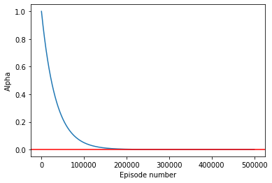
min(alpha_schedule2)0.001Running the Q-learning algorithm for different learning rate schedules
We start with the decay function that follows Equation 1. To get a full random policy, we set \(\epsilon = 1\). Note that this gives awful performance where the learning curve suggests it is hardly learning anything at all. However, wait until we try out a fully exploiting policy on the Q-value table learned during this run!
# K / N + K decay learning rate schedule
# fully random policy
plot_every = 100
alpha_schedule = create_alpha_schedule(num_episodes = 500_000, \
alpha_K = 5_000)
n_episodes = len(alpha_schedule)
fullrun = 0
if fullrun == 1:
Q_sarsamax, N_sarsamax, avg_scores, Qlist = q_learning(env, num_episodes = n_episodes, \
eps = 1,\
alpha_schedule = alpha_schedule, \
gamma = 0.95, \
plot_every = plot_every, \
verbose = True)
with open('cached/as1_Q_sarsamax.pkl', 'wb') as f:
dill.dump(Q_sarsamax, f)
with open('cached/as1_avg_scores.pkl', 'wb') as f:
dill.dump(avg_scores, f)
with open('cached/as1_Qlist.pkl', 'wb') as f:
dill.dump(Qlist, f)
else:
with open('cached/as1_Q_sarsamax.pkl', 'rb') as f:
Q_sarsamax = dill.load(f)
with open('cached/as1_avg_scores.pkl', 'rb') as f:
avg_scores = dill.load(f)
with open('cached/as1_Qlist.pkl', 'rb') as f:
Qlist = dill.load(f)
Q_as1_lasttable = [np.max(Q_sarsamax[key]) if key in Q_sarsamax \
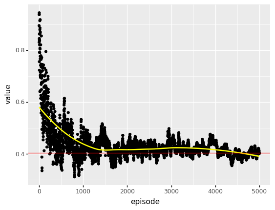
else 0 for key in np.arange(env.nS)]Here is the learning curve for this run of Q-learning:
# plot performance
plt.plot(np.linspace(0,n_episodes,len(avg_scores),endpoint=False), np.asarray(avg_scores))
plt.xlabel('Episode Number')
plt.ylabel('Average Reward (Over Next %d Episodes)' % plot_every)
plt.show()

print(('Best Average Reward over %d Episodes: ' % plot_every), np.max(avg_scores))
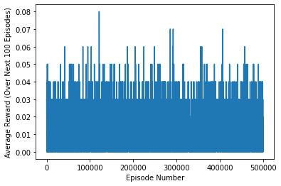
Best Average Reward over 100 Episodes: 0.08Pretty awfull huh? Now let us check out the performance of the learned Q-table:
fullrun = 0
runs = 100

if fullrun == 1:
    d_q = []
    for i in range(runs):
        avg_scores = test_performance(Q_sarsamax, env, num_episodes = 1000, \
                                   plot_every = 1000, verbose = False)
        d_q.append({'run': i,
                 'avg_score': np.mean(avg_scores)})
        print("\ri = {}/{}".format(i+1, runs), end="")
        sys.stdout.flush()

    d_qlearn = pd.DataFrame(d_q)
    d_qlearn.to_pickle('cached/scores_qlearn_0.95.pkl')
else:
    d_qlearn = pd.read_pickle('cached/scores_qlearn_0.95.pkl')
round(np.mean(d_qlearn.avg_score), 3)0.778Bam! Equal to the performance of the optimal policy found using Dynamic programming (sampling error (2x SD) is +/- 0.008). The random policy has actual learned Q-values that for a greedy policy result in optimal performance!
But what about convergence?
Ok, so Q-learning found an optimal policy. But did it converge?
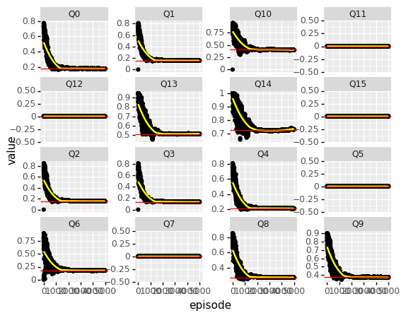
Our q_learning() function made a list of Q-tables while learning, adding a new table every 100 episodes. This gives us 5.000 datapoints for each Q-value, which we can plot to visually check for convergence.
As with the list of state-action tables above, It takes some datawrangling to get the list of Q-tables in a nice long pandas DataFrame suitable for plotting. This is hidden away in the list_to_df() function.
# 13s
dfm = list_to_df(Qlist)
#10 s
(p9.ggplot(data = dfm.loc[(dfm.episode > -1)], mapping = p9.aes(x = 'episode', y = 'value'))
+ p9.geom_point()
+ p9.geom_smooth(method = "loess", color = "yellow")
+ p9.geom_hline(data = df_true, mapping = p9.aes(yintercept = 'value'), color = 'red')
+ p9.facet_wrap("variable", scales = 'free_y')
+ p9.theme(subplots_adjust={'wspace':0.4}) # fix plotting issue
)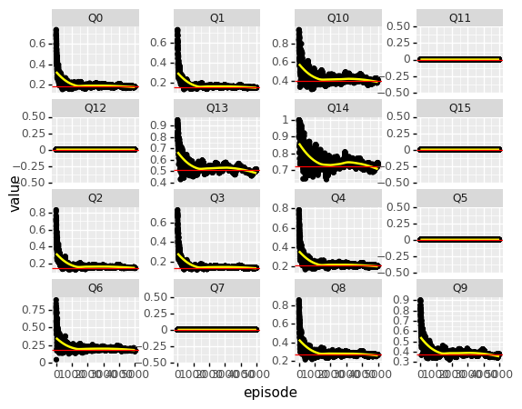
This looks good, lets zoom in at one of the more noisier Q-values, Q14.
In the learning schedule used, the lowest value for \(\alpha\) is 0.01.
At this value of the learning rate, there is still considerable variation around the true value.
(p9.ggplot(data = dfm.loc[(dfm.variable == 'Q10') & (dfm.episode > -1)], mapping = p9.aes(x = 'episode', y = 'value'))
    + p9.geom_point()
    + p9.geom_smooth(method = "loess", color = "yellow")
    + p9.geom_hline(data = df_true[df_true.variable == 'Q10'], mapping = p9.aes(yintercept = 'value'), color = 'red')
)
Suppose we did not know the true value of Q(S = 14), and wanted to estimate it using Q-learning. From the plot above, an obvious strategy is to average all the values in the tail of the learning rate schedule, say after episode 400.000.
# drop burn-in, then average Q-vals by variable
Q_est = (dfm.loc[dfm.episode > 4000]
         .groupby(['variable'])
         .mean()
        )

# convert to a 1D array sorted by Q-value
Q_est['sort_order'] = [int(str.replace(x, 'Q', '')) \
                       for x in Q_est.index.values]

Q_est = Q_est.sort_values(by=['sort_order'])

Q_est_as1 = Q_est['value'].values
Lets compare these with the final estimated values, and with true values:
Q_as1_lasttable = [np.max(Q_sarsamax[key]) if key in Q_sarsamax \
             else 0 for key in np.arange(env.nS)]

q_showdown = pd.DataFrame(
    {'q_est_as1': Q_est_as1,
     'q_est_as1_lasttable': Q_as1_lasttable,
     'q_true': V_pi_dc})
q_showdown['state'] = range(16)

q_showdown = pd.melt(q_showdown, ['state'])

(p9.ggplot(data = q_showdown, mapping = p9.aes(x = 'state', y = 'value', color = 'factor(variable)'))
+ p9.geom_point(size = 5, shape = 'x'))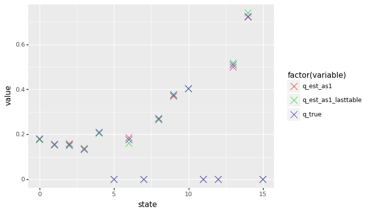
Pretty close! So here we see Q-learning finally delivering on its convergence promise.
And what about final values vs averaging? Averaging seems to have improved the estimates a bit. Note that we had to choose an averaging window based on eyeballing the learning curves for the separate Q-values.
Can we do even better? A learning rate schedule where alpha is lowered further would diminish the fluctuations around the true values, but at the risk of lowering it too fast and effectively freezing (or very slowly evolving) the Q-values at non-equilibrium values.
decay learning rate schedule variant II
The second formula decays \(\alpha\) to 0.001, ten times lower than the previous decay schedule:
# fully random policy

plot_every = 100

alpha_schedule2 = create_alpha_schedule2(num_episodes = 500_000, \
                                        alpha_decay = 0.99997)
n_episodes = len(alpha_schedule2)

fullrun = 0

if fullrun == 1:
    Q_sarsamax, N_sarsamax, avg_scores, Qlist = q_learning(env, num_episodes = n_episodes, \
                                                eps = 1,\
                                                alpha_schedule = alpha_schedule2, \
                                                gamma =  0.95, \
                                                plot_every = plot_every, \
                                                verbose = True)

    with open('cached/as2_Q_sarsamax.pkl', 'wb') as f:
        dill.dump(Q_sarsamax, f)
    with open('cached/as2_avg_scores.pkl', 'wb') as f:
        dill.dump(avg_scores, f)
    with open('cached/as2_Qlist.pkl', 'wb') as f:
        dill.dump(Qlist, f)
else:
    with open('cached/as2_Q_sarsamax.pkl', 'rb') as f:
        Q_sarsamax = dill.load(f)
    with open('cached/as2_avg_scores.pkl', 'rb') as f:
        avg_scores = dill.load(f)
    with open('cached/as2_Qlist.pkl', 'rb') as f:
        Qlist = dill.load(f)
dfm = list_to_df(Qlist)(p9.ggplot(data = dfm.loc[(dfm.episode > -1)], mapping = p9.aes(x = 'episode', y = 'value'))
+ p9.geom_point()
+ p9.geom_smooth(method = "loess", color = "yellow")
+ p9.geom_hline(data = df_true, mapping = p9.aes(yintercept = 'value'), color = 'red')
+ p9.facet_wrap("variable", scales = 'free_y')
+ p9.theme(subplots_adjust={'wspace':0.4})
)
Cleary, the fluctuations are reduced compared to the previous schedule. AND all Q-values still fluctuate around their true values, so it seems that this schedule is better with respect to finding the true values.
Let’s see if the accuracy of the estimated Q-values is indeed higher:
# drop burn-in, then average Q-vals by variable
Q_est = (dfm.loc[dfm.episode > 2000]
         .groupby(['variable'])
         .mean()
        )
# convert to 1d array sorted by state nr
Q_est['sort_order'] = [int(str.replace(x, 'Q', '')) \
                       for x in Q_est.index.values]

Q_est = Q_est.sort_values(by=['sort_order'])

Q_est_as2 = Q_est['value'].values

Q_as2_lasttable = [np.max(Q_sarsamax[key]) if key in Q_sarsamax \
             else 0 for key in np.arange(env.nS)]
q_showdown = pd.DataFrame(
{'Q_as2_lasttable': Q_as2_lasttable,
'q_est_as2': Q_est_as2,
'q_true': V_pi_dc})
q_showdown['state'] = range(16)
q_showdown = pd.melt(q_showdown, ['state'])
(p9.ggplot(data = q_showdown, mapping = p9.aes(x = 'state', y = 'value', color = 'factor(variable)'))
+ p9.geom_point(size = 5, shape = 'x'))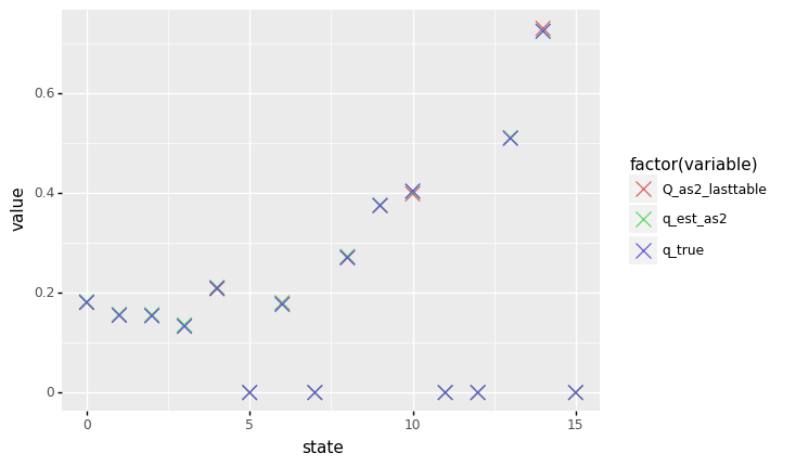
Boom! Now our \(Q^{*}_{a}\) estimates are really getting close to the true values. Clearly, the second learning rate schedule is able to learn the true Q-values compared to the first rate schedule, given the fixed amount of computation, in this case 500.000 episodes each.
Averaging out does not do much anymore, except for states 10 and 14, where it improves the estimates a tiny bit.
Wrapping up
In conclusion, we have seen that the common approach of using Q-learning with a constant learning rate and gradually decreasing the exploration rate, given sensible values and rates, will indeed find the optimal policy. However, this approach does not necessary converge to the true state-values. We have to tune the algorithm exactly the other way around: keep the exploration rate constant and sufficiently high, and decay the learning rate. For sufficiently low learning rates, averaging out the fluctuations does not meaningfully increase accuracy of the learned Q-values.
Gertjan Verhoeven
Data Scientist / Policy Advisor
Gertjan Verhoeven is a research scientist currently at the Dutch Healthcare Authority, working on health policy and statistical methods. Follow me on Twitter or Mastodon to receive updates on new blog posts. Statistics posts using R are featured on R-Bloggers.