
Improving a parametric regression model using machine learning
The idea is that comparing the predictions of an RF model with the predictions of an OLS model can inform us in what ways the OLS model fails to capture all non-linearities and interactions between the predictors. Subsequently, using partial dependence plots of the RF model can guide the modelling of the non-linearities in the OLS model. After this step, the discrepancies between the RF predictions and the OLS predictions should be caused by non-modeled interactions. Using an RF to predict the discrepancy itself can then be used to discover which predictors are involved in these interactions. We test this method on the classic Boston Housing dataset to predict median house values (medv). We indeed recover interactions that, as it turns, have already been found and documented in the literature.
Load packages
rm(list=ls())
#library(randomForest)
#library(party)
library(ranger)
library(data.table)
library(ggplot2)
library(MASS)

rdunif <- function(n,k) sample(1:k, n, replace = T)
Step 1: Run a RF on the Boston Housing set
my_ranger <- ranger(medv ~ ., data = Boston,
                                  importance = "permutation", num.trees = 500,
                                  mtry = 5, replace = TRUE)
Extract the permutation importance measure.
myres_tmp <- ranger::importance(my_ranger);
myres <- cbind(names(myres_tmp), myres_tmp,  i = 1)
#my_rownames <- row.names(myres)
myres <- data.table(myres)
setnames(myres, "V1", "varname")
setnames(myres, "myres_tmp", "MeanDecreaseAccuracy")
myres <- myres[, varname := as.factor(varname)]
myres <- myres[, MeanDecreaseAccuracy := as.numeric(MeanDecreaseAccuracy)]
myres <- myres[, i := as.integer(i)]
ggplot(myres,
aes(x = reorder(factor(varname), MeanDecreaseAccuracy), y = MeanDecreaseAccuracy)) +
geom_point() + coord_flip()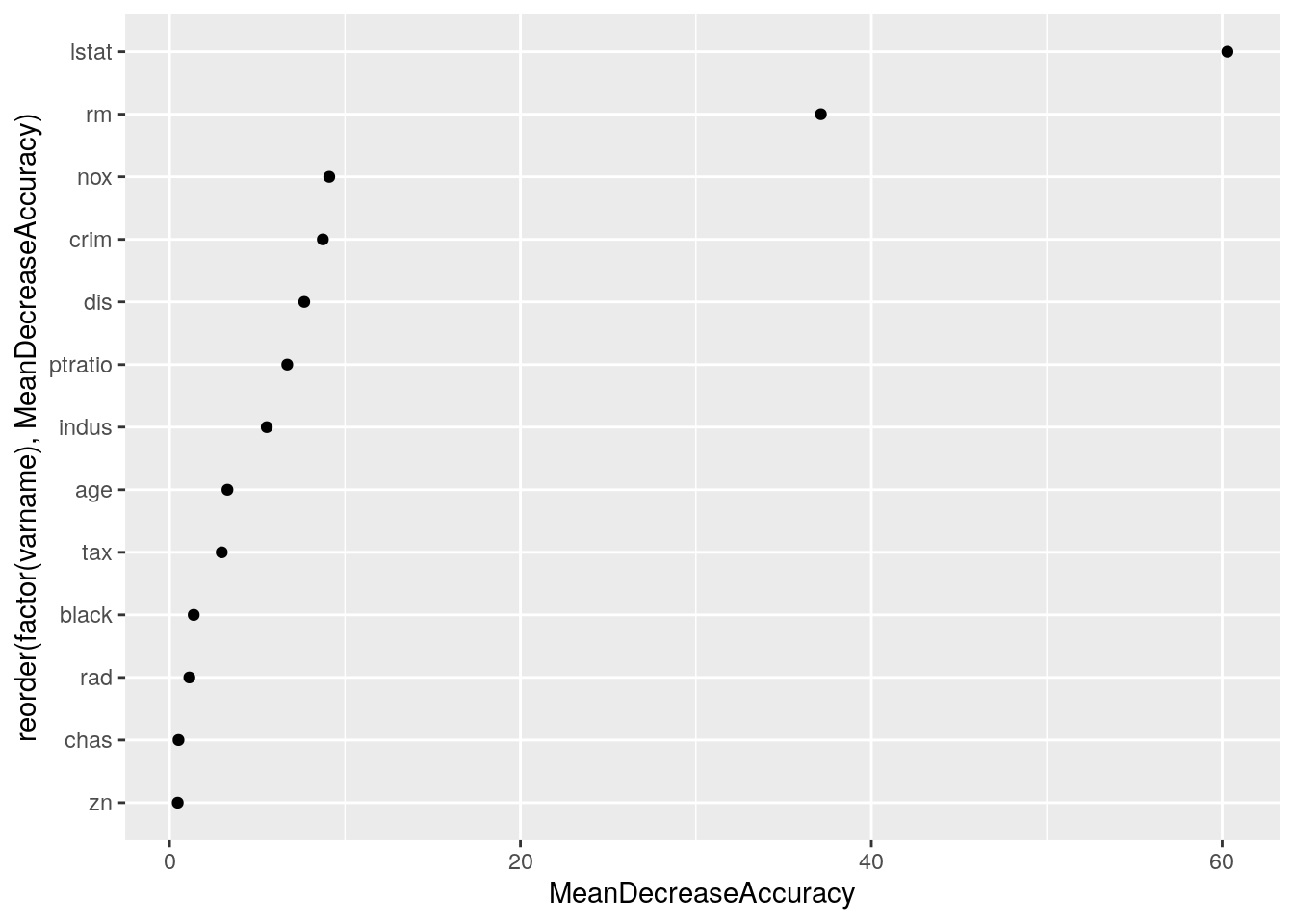
Fit an OLS to the Boston Housing
my_glm <- glm(medv ~., data = Boston,
              family = "gaussian")
Compare predictions of both models
pred_RF <- predict(my_ranger, data = Boston)
#pred_RF$predictions
pred_GLM <- predict(my_glm, data = Boston)
plot(pred_RF$predictions, pred_GLM)
abline(0, 1)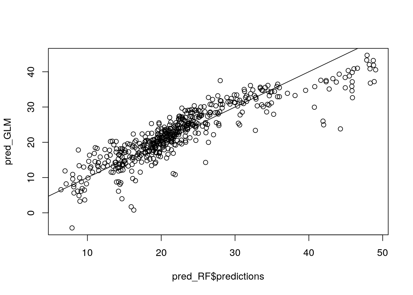 # Run a RF on the discrepancy
Discrepancy is defined as the difference between the predictions of both models for each observation.
pred_diff <- pred_RF$predictions - pred_GLM

my_ranger_diff <- ranger(Ydiff ~ . - medv, data = data.table(Ydiff = pred_diff, Boston),
                                  importance = "permutation", num.trees = 500,
                                  mtry = 5, replace = TRUE)
my_ranger_diff
## Ranger result
##
## Call:
## ranger(Ydiff ~ . - medv, data = data.table(Ydiff = pred_diff, Boston), importance = "permutation", num.trees = 500, mtry = 5, replace = TRUE)
##
## Type: Regression
## Number of trees: 500
## Sample size: 506
## Number of independent variables: 13
## Mtry: 5
## Target node size: 5
## Variable importance mode: permutation
## Splitrule: variance
## OOB prediction error (MSE): 5.151991
## R squared (OOB): 0.6674631It turns out the RF can "explain" 67% of these discrepancies.
myres_tmp <- ranger::importance(my_ranger_diff)
myres <- cbind(names(myres_tmp), myres_tmp,  i = 1)
#my_rownames <- row.names(myres)
myres <- data.table(myres)
setnames(myres, "V1", "varname")
setnames(myres, "myres_tmp", "MeanDecreaseAccuracy")
myres <- myres[, varname := as.factor(varname)]
myres <- myres[, MeanDecreaseAccuracy := as.numeric(MeanDecreaseAccuracy)]
myres <- myres[, i := as.integer(i)]
ggplot(myres,
aes(x = reorder(factor(varname), MeanDecreaseAccuracy), y = MeanDecreaseAccuracy)) +
geom_point() + coord_flip()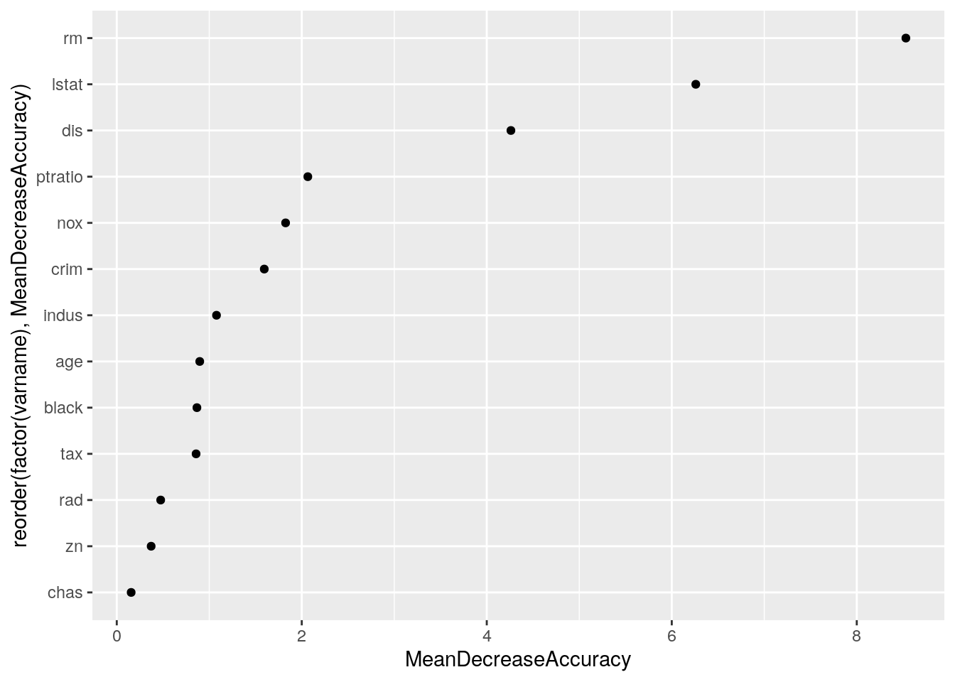
It turns out that rm and lstat are the variables that best predict the discrepancy.
my_glm_int <- glm(medv ~. + rm:lstat, data = Boston,
              family = "gaussian")
summary(my_glm_int)
##
## Call:
## glm(formula = medv ~ . + rm:lstat, family = "gaussian", data = Boston)
##
## Deviance Residuals:
## Min 1Q Median 3Q Max
## -21.5738 -2.3319 -0.3584 1.8149 27.9558
##
## Coefficients:
## Estimate Std. Error t value Pr(>|t|)
## (Intercept) 6.073638 5.038175 1.206 0.228582
## crim -0.157100 0.028808 -5.453 7.85e-08 ***
## zn 0.027199 0.012020 2.263 0.024083 *
## indus 0.052272 0.053475 0.978 0.328798
## chas 2.051584 0.750060 2.735 0.006459 **
## nox -15.051627 3.324807 -4.527 7.51e-06 ***
## rm 7.958907 0.488520 16.292 < 2e-16 ***
## age 0.013466 0.011518 1.169 0.242918
## dis -1.120269 0.175498 -6.383 4.02e-10 ***
## rad 0.320355 0.057641 5.558 4.49e-08 ***
## tax -0.011968 0.003267 -3.664 0.000276 ***
## ptratio -0.721302 0.115093 -6.267 8.06e-10 ***
## black 0.003985 0.002371 1.681 0.093385 .
## lstat 1.844883 0.191833 9.617 < 2e-16 ***
## rm:lstat -0.418259 0.032955 -12.692 < 2e-16 ***
## ---
## Signif. codes: 0 '***' 0.001 '**' 0.01 '*' 0.05 '.' 0.1 ' ' 1
##
## (Dispersion parameter for gaussian family taken to be 16.98987)
##
## Null deviance: 42716 on 505 degrees of freedom
## Residual deviance: 8342 on 491 degrees of freedom
## AIC: 2886
##
## Number of Fisher Scoring iterations: 2The interaction we have added is indeed highly significant.
Compare approximate out-of-sample prediction accuracy using AIC:
AIC(my_glm)## [1] 3027.609AIC(my_glm_int)## [1] 2886.043Indeed, the addition of the interaction greatly increases the prediction accuracy.
Repeat this process
pred_RF <- predict(my_ranger, data = Boston)
#pred_RF$predictions
pred_GLM <- predict(my_glm_int, data = Boston)

plot(pred_RF$predictions, pred_GLM)
abline(0, 1)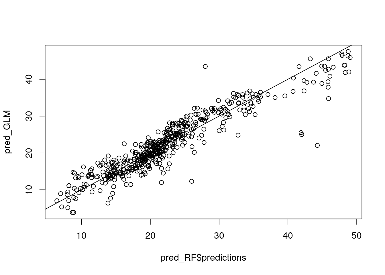
pred_diff <- pred_RF$predictions - pred_GLM

my_ranger_diff2 <- ranger(Ydiff ~ . - medv, data = data.table(Ydiff = pred_diff, Boston),
                                  importance = "permutation", num.trees = 500,
                                  mtry = 5, replace = TRUE)
my_ranger_diff2
## Ranger result
##
## Call:
## ranger(Ydiff ~ . - medv, data = data.table(Ydiff = pred_diff, Boston), importance = "permutation", num.trees = 500, mtry = 5, replace = TRUE)
##
## Type: Regression
## Number of trees: 500
## Sample size: 506
## Number of independent variables: 13
## Mtry: 5
## Target node size: 5
## Variable importance mode: permutation
## Splitrule: variance
## OOB prediction error (MSE): 5.604118
## R squared (OOB): 0.4399596myres_tmp <- ranger::importance(my_ranger_diff2)
myres <- cbind(names(myres_tmp), myres_tmp, i = 1)
#my_rownames <- row.names(myres)
myres <- data.table(myres)
setnames(myres, "V1", "varname")
setnames(myres, "myres_tmp", "MeanDecreaseAccuracy")
myres <- myres[, varname := as.factor(varname)]
myres <- myres[, MeanDecreaseAccuracy := as.numeric(MeanDecreaseAccuracy)]
myres <- myres[, i := as.integer(i)]ggplot(myres,
aes(x = reorder(factor(varname), MeanDecreaseAccuracy), y = MeanDecreaseAccuracy)) +
geom_point() + coord_flip()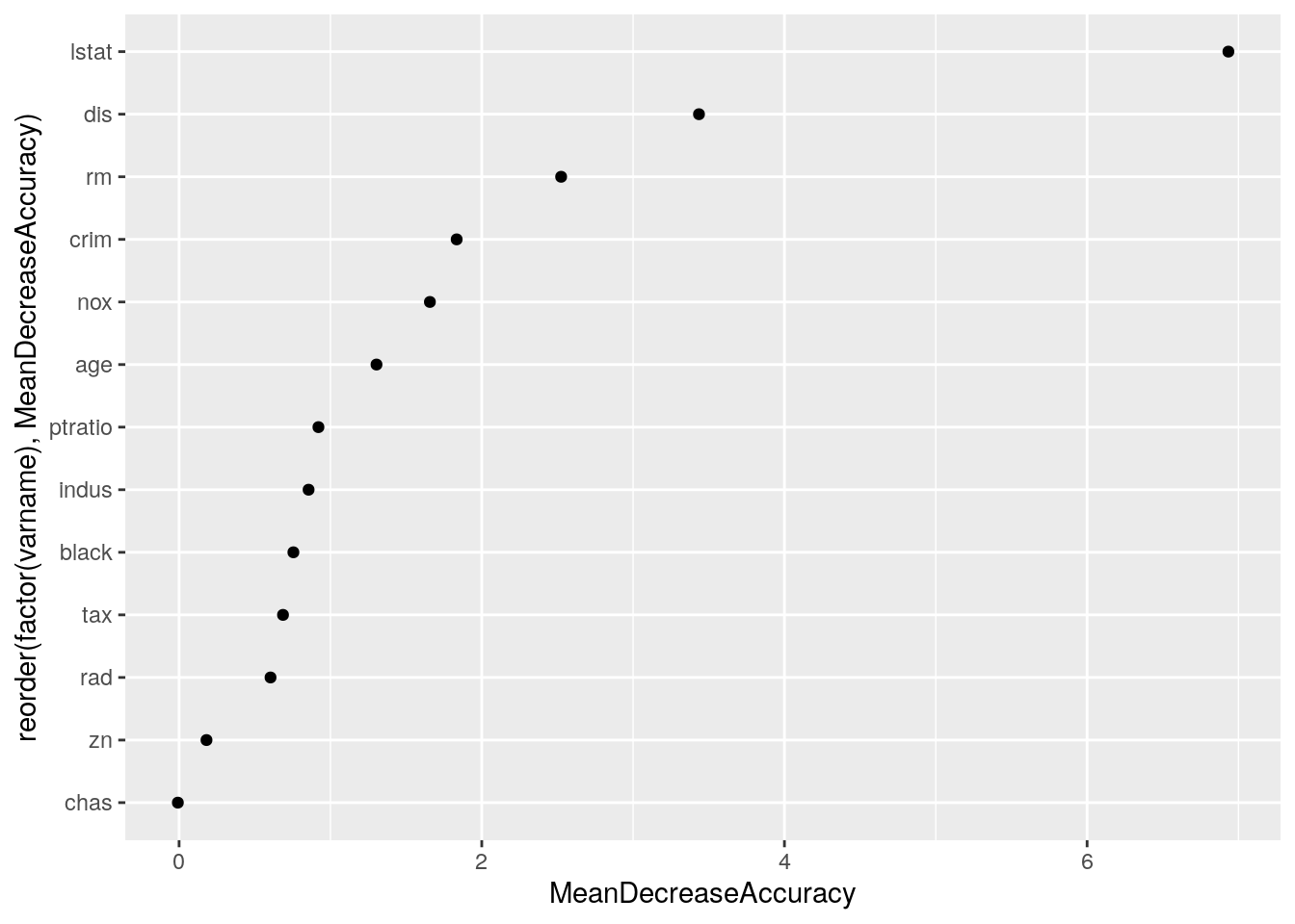
Now the variables that best predict the discrepancy are lstat and dis. Add these two variables as an interaction.
my_glm_int2 <- glm(medv ~. + rm:lstat + lstat:dis, data = Boston,
              family = "gaussian")
summary(my_glm_int2)
##
## Call:
## glm(formula = medv ~ . + rm:lstat + lstat:dis, family = "gaussian",
## data = Boston)
##
## Deviance Residuals:
## Min 1Q Median 3Q Max
## -23.3918 -2.2997 -0.4077 1.6475 27.6766
##
## Coefficients:
## Estimate Std. Error t value Pr(>|t|)
## (Intercept) 1.552991 5.107295 0.304 0.761201
## crim -0.139370 0.028788 -4.841 1.73e-06 ***
## zn 0.042984 0.012550 3.425 0.000667 ***
## indus 0.066690 0.052878 1.261 0.207834
## chas 1.760779 0.743688 2.368 0.018290 *
## nox -11.544280 3.404577 -3.391 0.000753 ***
## rm 8.640503 0.513593 16.824 < 2e-16 ***
## age -0.002127 0.012067 -0.176 0.860140
## dis -1.904982 0.268056 -7.107 4.22e-12 ***
## rad 0.304689 0.057000 5.345 1.39e-07 ***
## tax -0.011220 0.003228 -3.476 0.000554 ***
## ptratio -0.641380 0.115418 -5.557 4.51e-08 ***
## black 0.003756 0.002339 1.606 0.108924
## lstat 1.925223 0.190368 10.113 < 2e-16 ***
## rm:lstat -0.466947 0.034897 -13.381 < 2e-16 ***
## dis:lstat 0.076716 0.020009 3.834 0.000143 ***
## ---
## Signif. codes: 0 '***' 0.001 '**' 0.01 '*' 0.05 '.' 0.1 ' ' 1
##
## (Dispersion parameter for gaussian family taken to be 16.52869)
##
## Null deviance: 42716.3 on 505 degrees of freedom
## Residual deviance: 8099.1 on 490 degrees of freedom
## AIC: 2873.1
##
## Number of Fisher Scoring iterations: 2AIC(my_glm_int2)## [1] 2873.087AIC(my_glm_int)## [1] 2886.043We conclude that the second interaction also results in significant model improvement.
A more ambitious goal: Try and improve Harrison & Rubinfeld's model formula for Boston housing
So far, we assumed that all relationships are linear. Harrison and Rubinfeld have created a model without interactions, but with transformations to correct for skewness, heteroskedasticity etc. Let's see if we can improve upon this model equation by applying our method to search for interactions. Their formula predicts log(medv).
# Harrison and Rubinfeld (1978) model
my_glm_hr <- glm(log(medv) ~ I(rm^2) + age + log(dis) + log(rad) + tax + ptratio +
                     black + I(black^2) + log(lstat) + crim + zn + indus + chas + I(nox^2), data = Boston,
              family = "gaussian")

summary(my_glm_hr)
##
## Call:
## glm(formula = log(medv) ~ I(rm^2) + age + log(dis) + log(rad) +
## tax + ptratio + black + I(black^2) + log(lstat) + crim +
## zn + indus + chas + I(nox^2), family = "gaussian", data = Boston)
##
## Deviance Residuals:
## Min 1Q Median 3Q Max
## -0.73091 -0.09274 -0.00710 0.09800 0.78607
##
## Coefficients:
## Estimate Std. Error t value Pr(>|t|)
## (Intercept) 4.474e+00 1.579e-01 28.343 < 2e-16 ***
## I(rm^2) 6.634e-03 1.313e-03 5.053 6.15e-07 ***
## age 3.491e-05 5.245e-04 0.067 0.946950
## log(dis) -1.927e-01 3.325e-02 -5.796 1.22e-08 ***
## log(rad) 9.613e-02 1.905e-02 5.047 6.35e-07 ***
## tax -4.295e-04 1.222e-04 -3.515 0.000481 ***
## ptratio -2.977e-02 5.024e-03 -5.926 5.85e-09 ***
## black 1.520e-03 5.068e-04 3.000 0.002833 **
## I(black^2) -2.597e-06 1.114e-06 -2.331 0.020153 *
## log(lstat) -3.695e-01 2.491e-02 -14.833 < 2e-16 ***
## crim -1.157e-02 1.246e-03 -9.286 < 2e-16 ***
## zn 7.257e-05 5.034e-04 0.144 0.885430
## indus -1.943e-04 2.360e-03 -0.082 0.934424
## chas 9.180e-02 3.305e-02 2.777 0.005690 **
## I(nox^2) -6.566e-01 1.129e-01 -5.815 1.09e-08 ***
## ---
## Signif. codes: 0 '***' 0.001 '**' 0.01 '*' 0.05 '.' 0.1 ' ' 1
##
## (Dispersion parameter for gaussian family taken to be 0.03299176)
##
## Null deviance: 84.376 on 505 degrees of freedom
## Residual deviance: 16.199 on 491 degrees of freedom
## AIC: -273.48
##
## Number of Fisher Scoring iterations: 2my_ranger_log <- ranger(log(medv) ~ ., data = Boston,
importance = "permutation", num.trees = 500,
mtry = 5, replace = TRUE)pred_RF <- predict(my_ranger_log, data = Boston)
#pred_RF$predictions
pred_GLM <- predict(my_glm_hr, data = Boston)
plot(pred_RF$predictions, pred_GLM)
abline(0, 1)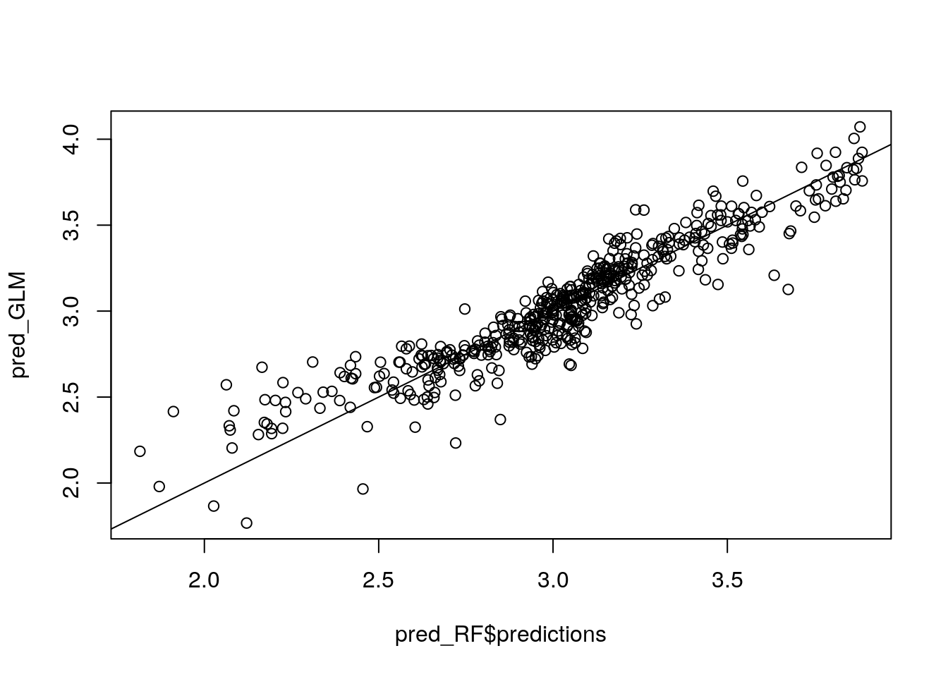
For low predicted values both models differ in a systematic way. This suggests that there exists a remaining pattern that is picked up by RF but not by the OLS model.
pred_diff <- pred_RF$predictions - pred_GLM

my_ranger_log_diff <- ranger(Ydiff ~ . - medv, data = data.table(Ydiff = pred_diff, Boston),
                                  importance = "permutation", num.trees = 500,
                                  mtry = 5, replace = TRUE)
my_ranger_log_diff
## Ranger result
##
## Call:
## ranger(Ydiff ~ . - medv, data = data.table(Ydiff = pred_diff, Boston), importance = "permutation", num.trees = 500, mtry = 5, replace = TRUE)
##
## Type: Regression
## Number of trees: 500
## Sample size: 506
## Number of independent variables: 13
## Mtry: 5
## Target node size: 5
## Variable importance mode: permutation
## Splitrule: variance
## OOB prediction error (MSE): 0.009132647
## R squared (OOB): 0.5268126The RF indicates that 54% of the discrepancy can be "explained" by RF.
myres_tmp <- ranger::importance(my_ranger_log_diff)
myres <- cbind(names(myres_tmp), myres_tmp,  i = 1)
#my_rownames <- row.names(myres)
myres <- data.table(myres)
setnames(myres, "V1", "varname")
setnames(myres, "myres_tmp", "MeanDecreaseAccuracy")
myres <- myres[, varname := as.factor(varname)]
myres <- myres[, MeanDecreaseAccuracy := as.numeric(MeanDecreaseAccuracy)]
myres <- myres[, i := as.integer(i)]
ggplot(myres,
aes(x = reorder(factor(varname), MeanDecreaseAccuracy), y = MeanDecreaseAccuracy)) +
geom_point() + coord_flip()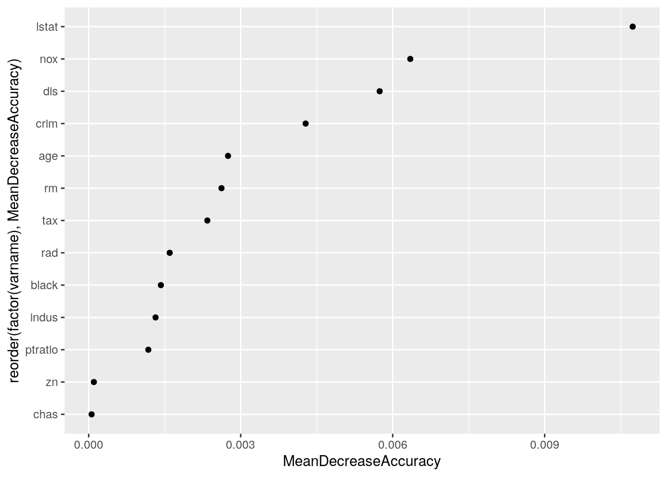
Add the top 2 vars as an interaction to their model equation.
my_glm_hr_int <- glm(log(medv) ~ I(rm^2) + age + log(dis) + log(rad) + tax + ptratio +
                     black + I(black^2) + log(lstat) + crim + zn + indus + chas + I(nox^2) +
                   lstat:nox, data = Boston,
              family = "gaussian")
summary(my_glm_hr_int)
##
## Call:
## glm(formula = log(medv) ~ I(rm^2) + age + log(dis) + log(rad) +
## tax + ptratio + black + I(black^2) + log(lstat) + crim +
## zn + indus + chas + I(nox^2) + lstat:nox, family = "gaussian",
## data = Boston)
##
## Deviance Residuals:
## Min 1Q Median 3Q Max
## -0.70340 -0.09274 -0.00665 0.10068 0.75004
##
## Coefficients:
## Estimate Std. Error t value Pr(>|t|)
## (Intercept) 4.243e+00 1.613e-01 26.304 < 2e-16 ***
## I(rm^2) 7.053e-03 1.286e-03 5.484 6.66e-08 ***
## age -3.146e-04 5.174e-04 -0.608 0.54354
## log(dis) -2.254e-01 3.317e-02 -6.795 3.15e-11 ***
## log(rad) 9.829e-02 1.862e-02 5.278 1.96e-07 ***
## tax -4.589e-04 1.196e-04 -3.838 0.00014 ***
## ptratio -2.990e-02 4.910e-03 -6.089 2.30e-09 ***
## black 1.445e-03 4.955e-04 2.917 0.00370 **
## I(black^2) -2.470e-06 1.089e-06 -2.268 0.02376 *
## log(lstat) -2.143e-01 3.989e-02 -5.373 1.20e-07 ***
## crim -1.046e-02 1.238e-03 -8.448 3.40e-16 ***
## zn 7.309e-04 5.099e-04 1.434 0.15234
## indus -8.166e-05 2.307e-03 -0.035 0.97178
## chas 8.746e-02 3.231e-02 2.707 0.00704 **
## I(nox^2) -3.618e-01 1.256e-01 -2.880 0.00415 **
## lstat:nox -2.367e-02 4.819e-03 -4.911 1.24e-06 ***
## ---
## Signif. codes: 0 '***' 0.001 '**' 0.01 '*' 0.05 '.' 0.1 ' ' 1
##
## (Dispersion parameter for gaussian family taken to be 0.03150809)
##
## Null deviance: 84.376 on 505 degrees of freedom
## Residual deviance: 15.439 on 490 degrees of freedom
## AIC: -295.79
##
## Number of Fisher Scoring iterations: 2AIC(my_glm_hr)## [1] -273.4788AIC(my_glm_hr_int)## [1] -295.7931This results in a significant improvement!
Repeat this procedure
pred_RF <- predict(my_ranger_log, data = Boston)
#pred_RF$predictions
pred_GLM <- predict(my_glm_hr_int, data = Boston)

plot(pred_RF$predictions, pred_GLM)
abline(0, 1)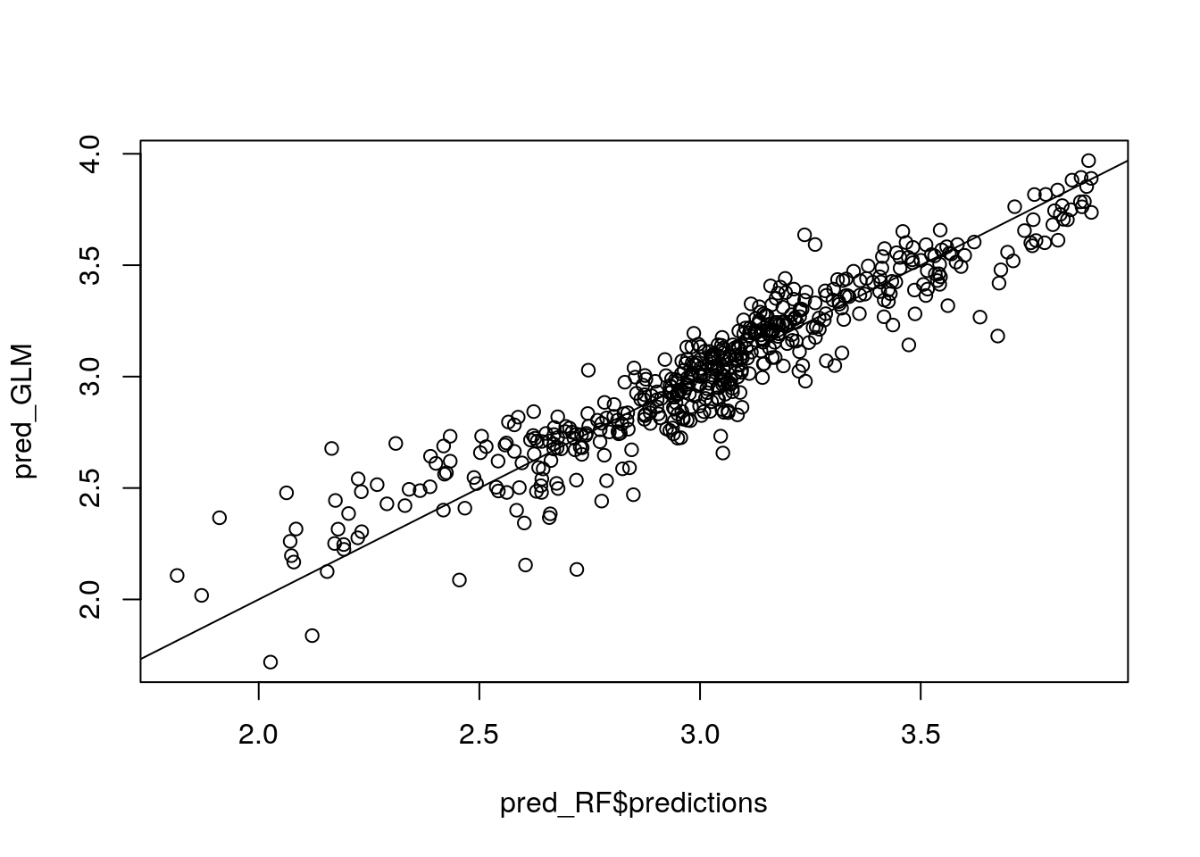
pred_diff <- pred_RF$predictions - pred_GLM

my_ranger_log_diff2 <- ranger(Ydiff ~ . - medv, data = data.table(Ydiff = pred_diff, Boston),
                                  importance = "permutation", num.trees = 500,
                                  mtry = 5, replace = TRUE)
my_ranger_log_diff2
## Ranger result
##
## Call:
## ranger(Ydiff ~ . - medv, data = data.table(Ydiff = pred_diff, Boston), importance = "permutation", num.trees = 500, mtry = 5, replace = TRUE)
##
## Type: Regression
## Number of trees: 500
## Sample size: 506
## Number of independent variables: 13
## Mtry: 5
## Target node size: 5
## Variable importance mode: permutation
## Splitrule: variance
## OOB prediction error (MSE): 0.008653356
## R squared (OOB): 0.5201821myres_tmp <- ranger::importance(my_ranger_log_diff2)
myres <- cbind(names(myres_tmp), myres_tmp, i = 1)
#my_rownames <- row.names(myres)
myres <- data.table(myres)
setnames(myres, "V1", "varname")
setnames(myres, "myres_tmp", "MeanDecreaseAccuracy")
myres <- myres[, varname := as.factor(varname)]
myres <- myres[, MeanDecreaseAccuracy := as.numeric(MeanDecreaseAccuracy)]
myres <- myres[, i := as.integer(i)]ggplot(myres,
aes(x = reorder(factor(varname), MeanDecreaseAccuracy), y = MeanDecreaseAccuracy)) +
geom_point() + coord_flip()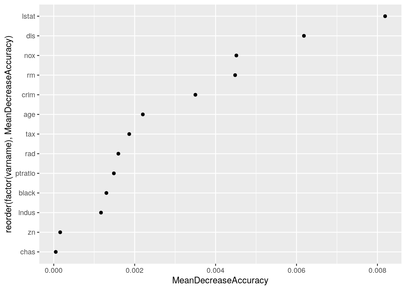
Now we add lstat and dis as an interaction.
my_glm_hr_int2 <- glm(log(medv) ~ I(rm^2) + age + log(dis) + log(rad) + tax + ptratio +
                     black + I(black^2) + log(lstat) + crim + zn + indus + chas + I(nox^2) +
                   lstat:nox + lstat:dis, data = Boston,
              family = "gaussian")
summary(my_glm_hr_int2)
##
## Call:
## glm(formula = log(medv) ~ I(rm^2) + age + log(dis) + log(rad) +
## tax + ptratio + black + I(black^2) + log(lstat) + crim +
## zn + indus + chas + I(nox^2) + lstat:nox + lstat:dis, family = "gaussian",
## data = Boston)
##
## Deviance Residuals:
## Min 1Q Median 3Q Max
## -0.70136 -0.08746 -0.00589 0.08857 0.76349
##
## Coefficients:
## Estimate Std. Error t value Pr(>|t|)
## (Intercept) 4.535e+00 1.712e-01 26.481 < 2e-16 ***
## I(rm^2) 7.498e-03 1.266e-03 5.924 5.94e-09 ***
## age -1.262e-03 5.504e-04 -2.293 0.02226 *
## log(dis) -4.065e-01 5.203e-02 -7.813 3.43e-14 ***
## log(rad) 9.668e-02 1.828e-02 5.290 1.85e-07 ***
## tax -4.622e-04 1.173e-04 -3.940 9.35e-05 ***
## ptratio -2.640e-02 4.881e-03 -5.409 9.93e-08 ***
## black 1.313e-03 4.871e-04 2.696 0.00727 **
## I(black^2) -2.172e-06 1.071e-06 -2.029 0.04303 *
## log(lstat) -3.181e-01 4.553e-02 -6.987 9.23e-12 ***
## crim -1.049e-02 1.215e-03 -8.635 < 2e-16 ***
## zn 9.078e-04 5.019e-04 1.809 0.07108 .
## indus -2.733e-04 2.264e-03 -0.121 0.90395
## chas 7.166e-02 3.191e-02 2.246 0.02515 *
## I(nox^2) -2.569e-01 1.255e-01 -2.048 0.04113 *
## lstat:nox -2.729e-02 4.798e-03 -5.689 2.21e-08 ***
## lstat:dis 3.906e-03 8.754e-04 4.462 1.01e-05 ***
## ---
## Signif. codes: 0 '***' 0.001 '**' 0.01 '*' 0.05 '.' 0.1 ' ' 1
##
## (Dispersion parameter for gaussian family taken to be 0.03033711)
##
## Null deviance: 84.376 on 505 degrees of freedom
## Residual deviance: 14.835 on 489 degrees of freedom
## AIC: -313.99
##
## Number of Fisher Scoring iterations: 2AIC(my_glm_hr_int2)## [1] -313.9904AIC(my_glm_hr_int)## [1] -295.7931And again we find an improvement in model fit.
Have these interactions already been reported on in the literature?
Tom Minka reports on his website an analysis of interactions in the Boston Housing set:
(http://alumni.media.mit.edu/~tpminka/courses/36-350.2001/lectures/day30/) > summary(fit3) Coefficients: Estimate Std. Error t value Pr(>|t|) (Intercept) -227.5485 49.2363 -4.622 4.87e-06 *** lstat 50.8553 20.3184 2.503 0.012639 * rm 38.1245 7.0987 5.371 1.21e-07 *** dis -16.8163 2.9174 -5.764 1.45e-08 *** ptratio 14.9592 2.5847 5.788 1.27e-08 *** lstat:rm -6.8143 3.1209 -2.183 0.029475 * lstat:dis 4.8736 1.3940 3.496 0.000514 *** lstat:ptratio -3.3209 1.0345 -3.210 0.001412 ** rm:dis 2.0295 0.4435 4.576 5.99e-06 *** rm:ptratio -1.9911 0.3757 -5.299 1.76e-07 *** lstat:rm:dis -0.5216 0.2242 -2.327 0.020364 * lstat:rm:ptratio 0.3368 0.1588 2.121 0.034423 *
Rob mcCulloch, using BART (bayesian additive regression trees) also examines interactions in the Boston Housing data. There the co-occurence within trees is used to discover interactions:
The second, interaction detection, uncovers which pairs of variables interact in analogous fashion by keeping track of the percentage of trees in the sum in which both variables occur. This exploits the fact that a sum-of-trees model captures an interaction between xi and xj by using them both for splitting rules in the same tree.
http://www.rob-mcculloch.org/some_papers_and_talks/papers/working/cgm_as.pdf

Conclusion
We conclude that this appears a fruitfull approach to at least discovering where a regression model can be improved.
Gertjan Verhoeven
Data Scientist / Policy Advisor
Gertjan Verhoeven is a research scientist currently at the Dutch Healthcare Authority, working on health policy and statistical methods. Follow me on Twitter or Mastodon to receive updates on new blog posts. Statistics posts using R are featured on R-Bloggers.