
The validation set approach in caret
In this blog post, we explore how to implement the validation set approach in caret. This is the most basic form of the train/test machine learning concept. For example, the classic machine learning textbook "An introduction to Statistical Learning" uses the validation set approach to introduce resampling methods.
In practice, one likes to use k-fold Cross validation, or Leave-one-out cross validation, as they make better use of the data. This is probably the reason that the validation set approach is not one of caret's preset methods.
But for teaching purposes it would be very nice to have a caret implementation.
This would allow for an easy demonstration of the variability one gets when choosing different partionings. It also allows direct demonstration of why k-fold CV is superior to the validation set approach with respect to bias/variance.
We pick the BostonHousing dataset for our example code.
# Boston Housing
knitr::kable(head(Boston))| crim | zn | indus | chas | nox | rm | age | dis | rad | tax | ptratio | black | lstat | medv |
|---|---|---|---|---|---|---|---|---|---|---|---|---|---|
| 0.00632 | 18 | 2.31 | 0 | 0.538 | 6.575 | 65.2 | 4.0900 | 1 | 296 | 15.3 | 396.90 | 4.98 | 24.0 |
| 0.02731 | 0 | 7.07 | 0 | 0.469 | 6.421 | 78.9 | 4.9671 | 2 | 242 | 17.8 | 396.90 | 9.14 | 21.6 |
| 0.02729 | 0 | 7.07 | 0 | 0.469 | 7.185 | 61.1 | 4.9671 | 2 | 242 | 17.8 | 392.83 | 4.03 | 34.7 |
| 0.03237 | 0 | 2.18 | 0 | 0.458 | 6.998 | 45.8 | 6.0622 | 3 | 222 | 18.7 | 394.63 | 2.94 | 33.4 |
| 0.06905 | 0 | 2.18 | 0 | 0.458 | 7.147 | 54.2 | 6.0622 | 3 | 222 | 18.7 | 396.90 | 5.33 | 36.2 |
| 0.02985 | 0 | 2.18 | 0 | 0.458 | 6.430 | 58.7 | 6.0622 | 3 | 222 | 18.7 | 394.12 | 5.21 | 28.7 |
Our model is predicting medv (Median house value) using predictors indus and chas in a multiple linear regression. We split the data in half, 50% for fitting the model, and 50% to use as a validation set.
Stratified sampling vs random sampling
To check if we understand what caret does, we first implement the validation set approach ourselves. To be able to compare, we need exactly the same data partitions for our manual approach and the caret approach. As caret requires a particular format (a named list of sets of train indices) we conform to this standard. However, all caret partitioning functions seem to perform stratified random sampling. This means that it first partitions the data in equal sized groups based on the outcome variable, and then samples at random within those groups to partitions that have similar distributions for the outcome variable.
This not desirable for teaching, as it adds more complexity. In addition, it would be nice to be able to compare stratified vs. random sampling.
We therefore write a function that generates truly random partitions of the data. We let it generate partitions in the format that trainControl likes.
# internal function from caret package, needed to play nice with resamples()
prettySeq <- function(x) paste("Resample", gsub(" ", "0", format(seq(along = x))), sep = "")

createRandomDataPartition <- function(y, times, p) {
  vec <- 1:length(y)
  n_samples <- round(p * length(y))

  result <- list()
  for(t in 1:times){
    indices <- sample(vec, n_samples, replace = FALSE)
    result[[t]] <- indices
    #names(result)[t] <- paste0("Resample", t)
  }
  names(result) <- prettySeq(result)
  result
}

createRandomDataPartition(1:10, times = 2, p = 0.5)
## $Resample1
## [1] 4 3 7 9 10
##
## $Resample2
## [1] 8 6 1 7 10The validation set approach without caret
Here is the validation set approach without using caret. We create a single random partition of the data in train and validation set, fit the model on the training data, predict on the validation data, and calculate the RMSE error on the test predictions.
set.seed(1234)
parts <- createRandomDataPartition(Boston$medv, times = 1, p = 0.5)

train <- parts$Resample1

# fit ols on train data
lm.fit <- lm(medv ~ indus + chas , data = Boston[train,])

# predict on held out data
preds <- predict(lm.fit, newdata = Boston[-train,])

# calculate RMSE validation error
sqrt(mean((preds - Boston[-train,]$medv)^2))
## [1] 7.930076If we feed caret the same data partition, we expect exactly the same test error for the held-out data. Let's find out!
The validation set approach in caret
Now we use the caret package. Regular usage requires two function calls, one to trainControl to control the resampling behavior, and one to train to do the actual model fitting and prediction generation.
As the validation set approach is not one of the predefined methods, we need to make use of the index argument to explicitely define the train partitions outside of caret. It automatically predicts on the records that are not contained in the train partitions.
The index argument plays well with the createDataPartition (Stratfied sampling) and createRandomDataPartition (our own custom function that performs truly random sampling) functions, as these functions both generate partitions in precisely the format that index wants: lists of training set indices.
In the code below, we generate four different 50/50 partitions of the data.
We set savePredictions to TRUE to be able to verify the calculated metrics such as the test RMSE.
set.seed(1234)

# create four partitions
parts <- createRandomDataPartition(Boston$medv, times = 4, p = 0.5)

ctrl <- trainControl(method = "repeatedcv",
                     ## The method doesn't matter
                     ## since we are defining the resamples
                     index= parts,
                     ##verboseIter = TRUE,
                     ##repeats = 1,
                     savePredictions = TRUE
                     ##returnResamp = "final"
                     )
Now we can run caret and fit the model four times:
res <- train(medv ~ indus + chas, data = Boston, method = "lm",
             trControl = ctrl)

res
## Linear Regression
##
## 506 samples
## 2 predictor
##
## No pre-processing
## Resampling: Cross-Validated (10 fold, repeated 1 times)
## Summary of sample sizes: 253, 253, 253, 253
## Resampling results:
##
## RMSE Rsquared MAE
## 7.906538 0.2551047 5.764773
##
## Tuning parameter 'intercept' was held constant at a value of TRUEFrom the result returned by train we can verify that it has fitted a model on four different datasets, each of size 253. By default it reports the average test error over the four validation sets. We can also extract the four individual test errors:
# strangely enough, resamples() always wants at least two train() results
# see also the man page for resamples()
resamples <- resamples(list(MOD1 = res,
                            MOD2 = res))

resamples$values$`MOD1~RMSE`
## [1] 7.930076 8.135428 7.899054 7.661595# check that we recover the RMSE reported by train() in the Resampling results
mean(resamples$values$`MOD1~RMSE`)## [1] 7.906538summary(resamples)##
## Call:
## summary.resamples(object = resamples)
##
## Models: MOD1, MOD2
## Number of resamples: 4
##
## MAE
## Min. 1st Qu. Median Mean 3rd Qu. Max. NA's
## MOD1 5.516407 5.730172 5.809746 5.764773 5.844347 5.923193 0
## MOD2 5.516407 5.730172 5.809746 5.764773 5.844347 5.923193 0
##
## RMSE
## Min. 1st Qu. Median Mean 3rd Qu. Max. NA's
## MOD1 7.661595 7.839689 7.914565 7.906538 7.981414 8.135428 0
## MOD2 7.661595 7.839689 7.914565 7.906538 7.981414 8.135428 0
##
## Rsquared
## Min. 1st Qu. Median Mean 3rd Qu. Max. NA's
## MOD1 0.2339796 0.2377464 0.2541613 0.2551047 0.2715197 0.2781167 0
## MOD2 0.2339796 0.2377464 0.2541613 0.2551047 0.2715197 0.2781167 0Note that the RMSE value for the first train/test partition is exactly equal to our own implementation of the validation set approach. Awesome.
Validation set approach: stratified sampling versus random sampling
Since we now know what we are doing, let's perform a simulation study to compare stratified random sampling with truly random sampling, using the validation set approach, and repeating this proces say a few thousand times to get a nice distribution of test errors.
# simulation settings
n_repeats <- 3000
train_fraction <- 0.8
First we fit the models on the random sampling data partitions:
set.seed(1234)
parts <- createRandomDataPartition(Boston$medv, times = n_repeats, p = train_fraction)

ctrl <- trainControl(method = "repeatedcv",  ## The method doesn't matter
                     index= parts,
                     savePredictions = TRUE
                     )

rand_sampl_res <- train(medv ~ indus + chas, data = Boston, method = "lm",
             trControl = ctrl)

rand_sampl_res
## Linear Regression
##
## 506 samples
## 2 predictor
##
## No pre-processing
## Resampling: Cross-Validated (10 fold, repeated 1 times)
## Summary of sample sizes: 405, 405, 405, 405, 405, 405, ...
## Resampling results:
##
## RMSE Rsquared MAE
## 7.868972 0.2753001 5.790874
##
## Tuning parameter 'intercept' was held constant at a value of TRUENext, we fit the models on the stratified sampling data partitions:
set.seed(1234)
parts <- createDataPartition(Boston$medv, times = n_repeats, p = train_fraction, list = T)

ctrl <- trainControl(method = "repeatedcv",  ## The method doesn't matter
                     index= parts,
                     savePredictions = TRUE
                     )

strat_sampl_res <- train(medv ~ indus + chas, data = Boston, method = "lm",
             trControl = ctrl)

strat_sampl_res
## Linear Regression
##
## 506 samples
## 2 predictor
##
## No pre-processing
## Resampling: Cross-Validated (10 fold, repeated 1 times)
## Summary of sample sizes: 407, 407, 407, 407, 407, 407, ...
## Resampling results:
##
## RMSE Rsquared MAE
## 7.83269 0.277719 5.769507
##
## Tuning parameter 'intercept' was held constant at a value of TRUEThen, we merge the two results to compare the distributions:
resamples <- resamples(list(RAND = rand_sampl_res,
                          STRAT = strat_sampl_res))
Analyzing caret resampling results
We now analyse our resampling results. We can use the summary method on our resamples object:
summary(resamples)##
## Call:
## summary.resamples(object = resamples)
##
## Models: RAND, STRAT
## Number of resamples: 3000
##
## MAE
## Min. 1st Qu. Median Mean 3rd Qu. Max. NA's
## RAND 4.406326 5.475846 5.775077 5.790874 6.094820 7.582886 0
## STRAT 4.401729 5.477664 5.758201 5.769507 6.058652 7.356133 0
##
## RMSE
## Min. 1st Qu. Median Mean 3rd Qu. Max. NA's
## RAND 5.328128 7.323887 7.847369 7.868972 8.408855 10.78024 0
## STRAT 5.560942 7.304199 7.828765 7.832690 8.328966 10.44186 0
##
## Rsquared
## Min. 1st Qu. Median Mean 3rd Qu. Max. NA's
## RAND 0.06982417 0.2259553 0.2733762 0.2753001 0.3249820 0.5195017 0
## STRAT 0.05306875 0.2263577 0.2752015 0.2777190 0.3277577 0.4977015 0We can also use the plot function provided by the caret package. It plots the mean of our performance metric (RMSE), as well as estimation uncertainty of this mean. Note that the confidence intervals here are based on a normal approximation (One sample t-test).
# caret:::ggplot.resamples
# t.test(resamples$values$`RAND~RMSE`)
ggplot(resamples, metric = "RMSE") 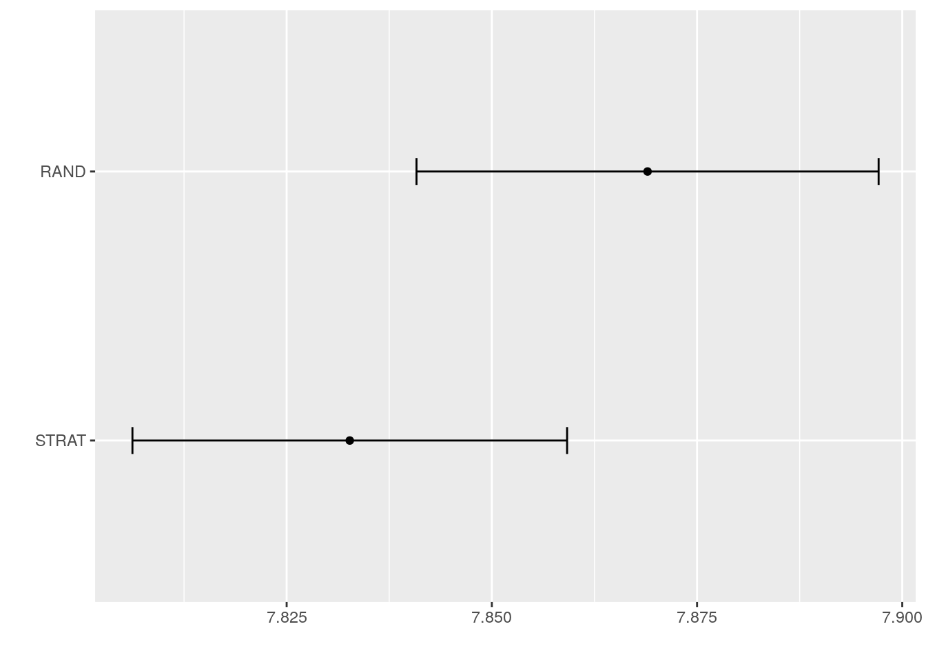
My personal preference is to more directly display both distributions. This is done by bwplot() (caret does not have ggplot version of this function).
bwplot(resamples, metric = "RMSE")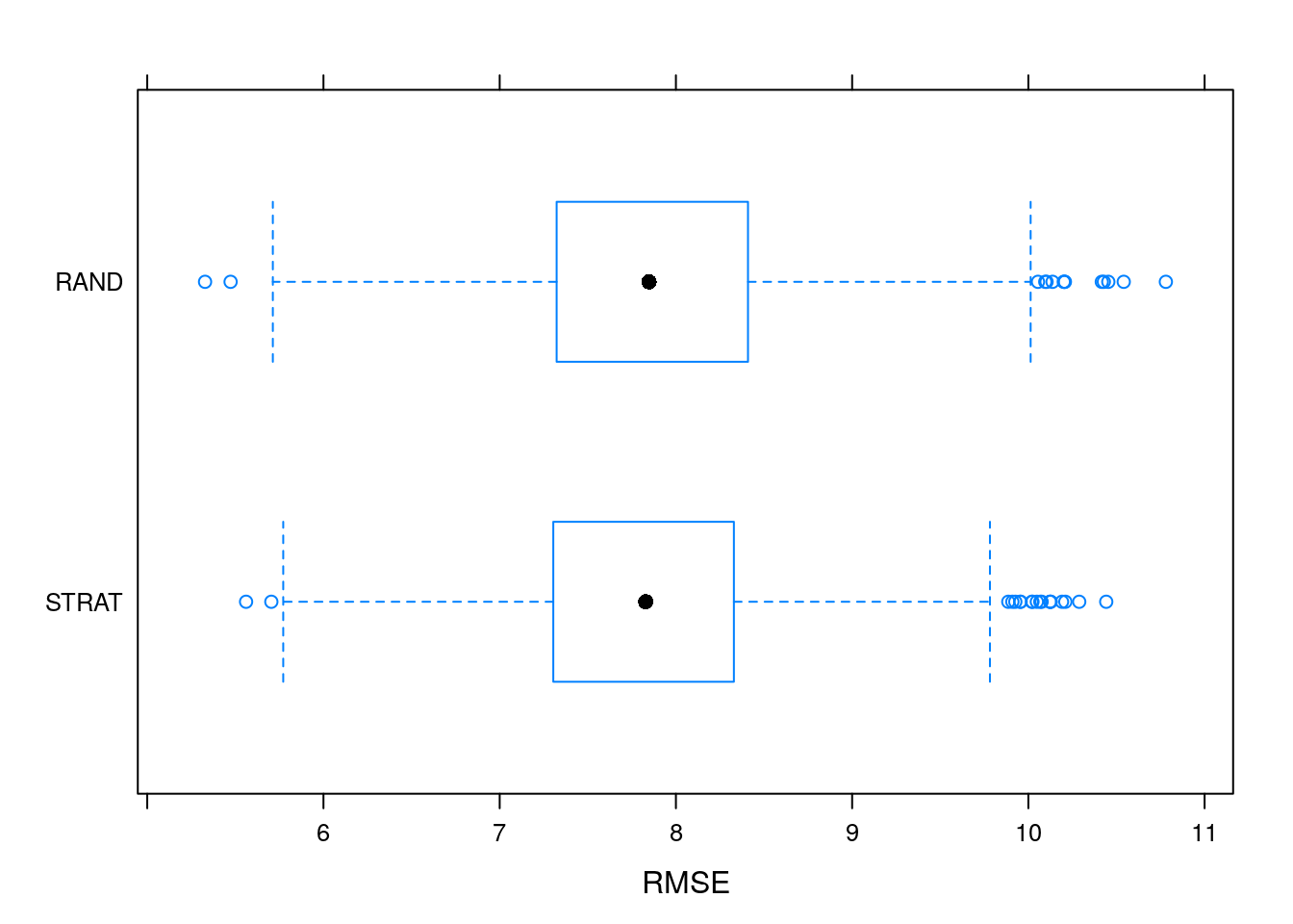
It does seems that stratified sampling paints a slightly more optimistic picture of the test error when compared to truly random sampling. However, we can also see that random sampling has somewhat higher variance when compared to stratified sampling.
Based on these results, it seems like stratified sampling is indeed a reasonable default setting for caret.
Update: LGOCV
set.seed(1234)


ctrl <- trainControl(method = "LGOCV",  ## The method doesn't matter
                     repeats = n_repeats,
                     number = 1,
                     p = 0.5,
                     savePredictions = TRUE
                     )
## Warning: `repeats` has no meaning for this resampling method.lgocv_res <- train(medv ~ indus + chas, data = Boston, method = "lm",
trControl = ctrl)
lgocv_res## Linear Regression
##
## 506 samples
## 2 predictor
##
## No pre-processing
## Resampling: Repeated Train/Test Splits Estimated (1 reps, 50%)
## Summary of sample sizes: 254
## Resampling results:
##
## RMSE Rsquared MAE
## 8.137926 0.2389733 5.763309
##
## Tuning parameter 'intercept' was held constant at a value of TRUEGertjan Verhoeven
Data Scientist / Policy Advisor
Gertjan Verhoeven is a research scientist currently at the Dutch Healthcare Authority, working on health policy and statistical methods. Follow me on Twitter or Mastodon to receive updates on new blog posts. Statistics posts using R are featured on R-Bloggers.