Optimal performance with Random Forests: does feature selection beat tuning?

Why Random Forest is my favorite ML algorithm

The Random Forest algorithm (Breiman 2001) is my favorite ML algorithm for cross-sectional, tabular data. Thanks to Marvin Wright a fast and reliable implementation exists for R called ranger(Wright and Ziegler 2017). For tabular data, RF seems to offer the highest value per unit of compute compared to other popular ML methods, such as Deep learning or Gradient Boosting algorithms such as XGBoost. In this setting, predictive performance is often on par with Deep Learning or Gradient boosting (Svetnik et al. 2005; Xu et al. 2021). For classification prediction models, it has been shown to outperform logistic regression (Couronné, Probst, and Boulesteix 2018).

The Random Forest algorithm can provide a quick benchmark for the predictive performance of a set of predictors, that is hard to beat with models that explicitly formulate a interpretable model of a dependent variable, for example a linear regression model with interactions and non-linear transformations of the predictors. For a great talk on the Random Forest method, check out Prof. Marvin Wright’s UseR talk from 2019 on YouTube.

But it is not perfect: the effect of irrelevant variables

In that talk, Marvin Wright discusses the common claim that “Random Forest works well on high-dimensional data”. High-dimensional data is common in genetics, when we have say complete genomes for only a handful of subjects. The suggestion is that RF can be used on small datasets with lots of (irrelevant / noise) features without having to do variable selection first.

To check this claim, Wright shows that RF performance is unaffected by adding 100 noise variables to the iris dataset, a simple example classification problem with three different species. Because RF uses decision trees, it performs “automatic” feature (predictor / variable) selection as part of the model building process. This property of the algorithm is used to explain this result. A tree model will simply ignore the noise predictors and choose the relevant predictors instead.

See the accompanying R notebook prep_and_fit.Rmd that contains all the simulations I performed for this blog post. It also includes the simulation on the iris dataset:

fit_list <- readRDS("rf_rfe_post/fitlist.rds")
fit_list$algo <- paste0(fit_list$method, "_mtry_", fit_list$mtry)

fit_list %>% filter(ds_group == "df_iris" & algo == "ranger_mtry_default")

## # A tibble: 2 × 17
##   model_id method mtry    ds_id ds_name      ds_group target  forest_type n_obs
##      <int> <chr>  <chr>   <int> <chr>        <chr>    <chr>   <chr>       <int>
## 1        1 ranger default     4 df_iris      df_iris  Species class         150
## 2        1 ranger default     5 df_iris_N100 df_iris  Species class         150
## # … with 8 more variables: n_features <dbl>, fit_id <int>, performance <dbl>,
## #   algo <chr>, performance_lower <dbl>, performance_upper <dbl>,
## #   performance_boot <dbl>, performance_boot_corr <dbl>

source("rf_rfe_post/plot_performance.R")

plot_performance(data = fit_list %>% filter(ds_group == "df_iris" & algo == "ranger_mtry_default"),
                 axis_label = "Accuracy (% correct)",
                 plot_title = "Adding 100 noise variables to the iris dataset", 
                 facet_var = "algo", x_var = "ds_name")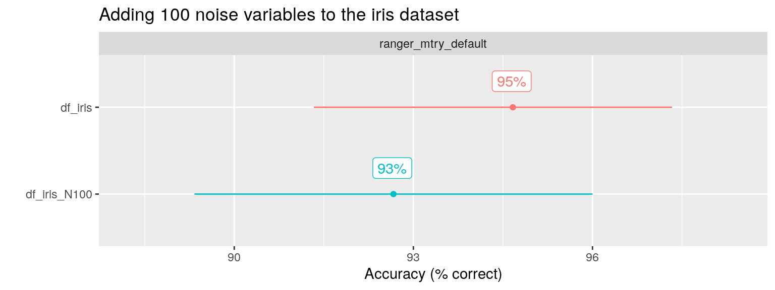

Indeed, the performance (here i looked at Accuracy as percentage of observations correctly classified) is hardly affected.

(As we will be doing a lot of model performance comparison, I added 90% bootstrapped confidence intervals for the performance metrics used in this post. This interval was generated from 1000 bootstrapped values of R2 using resampling on the vectors of (out-of-bag) predictions and the observed y-values (This deserves its own future blog post, if you can’t wait just check the prep_and_fit.Rmd notebook on my Github)).

However, a counter example, where adding irrelevant features does hurt performance, is quickly found. In Chapter 20 of the documentation of caret, a popular ML package in R, Max Kuhn introduces the regression problem Friedman 1 to illustrate the problem, as well as a possible solution. See for a different example in the literature (Genuer, Poggi, and Tuleau-Malot 2010).

mlbench.friedman1() simulates the regression problem Friedman 1. Inputs are 10 independent variables uniformly distributed on the interval [0,1], only 5 out of these 10 are actually used in the formula to generate the dependent variable \(y\):

\(y = 10 sin(\pi x_1 x_2) + 20 (x_3 - 0.5)^2 + 10 x_4 + 5 x_5 + \epsilon\)

where \(\epsilon\) is distributed \(Normal(0, 1)\).

(source: (Friedman 1991; Breiman 1996))

Kuhn added 40 more noise variables to the dataset and simulated N = 100 observations. Now only five predictors contain signal, whereas the other 45 contain noise. Random Forest with its default setting of mtry shows poor performance, and only after performing feature selection (removing the irrelevant variables) optimal performance is achieved (see below for more about feature selection, here the point is the reduced performance after adding noise).

I also reproduced this analysis, but with N = 1000 and with 0, 100 and 500 additional noise variables added (instead of 40).

plot_performance(data = fit_list %>% filter(ds_group == "df_friedman1" & algo %in% c("ranger_mtry_default")),
                 axis_label = "R-squared (%)",
                 plot_title = "Adding increasing amount of noise to the Friedman 1 dataset", facet_var = "algo", x_var = "ds_name")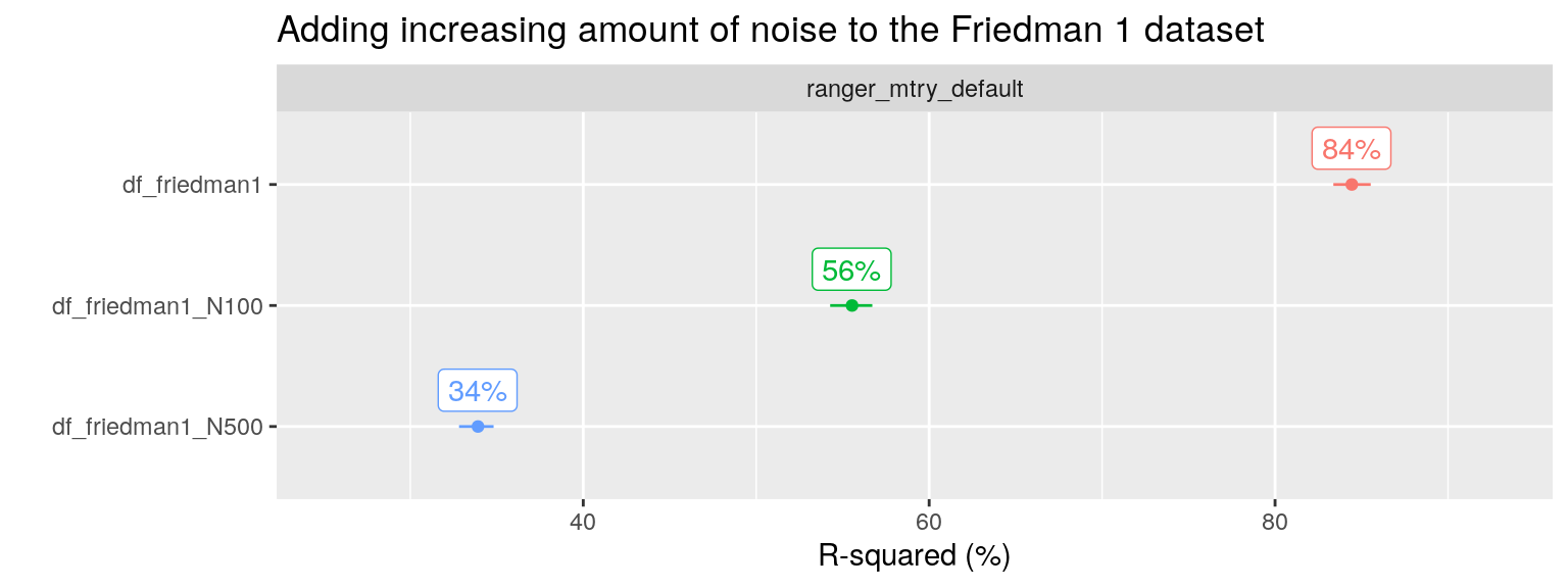

We can check the optimal performance by only including the relevant predictors \(x_1, x_2,x_3,x_4, x_5\) in the RF algorithm: such a model has an R-squared of around 88% (not shown). RF including both signal and five noise predictors, the original Friedman 1 problem, shows a slight drop in performance to 84% with the default mtry value. After including an additional 100 noise variables, performance drops further to 56%. And if we add 500 instead of 100 additional noise variables, performance drops even further to 34% R2.

So how to solve this? In this blog post, I will compare both RF hyperparameter tuning and feature selection in the presence of many irrelevant features.

Tuning RF or removing the irrelevant features?

It seems that most practical guidance to improve RF performance is on tuning the algorithm hyperparameters, arguing that Random Forest as a tree-based method has built-in feature selection, alleviating the need to remove irrelevant features.

This is demonstrated by the many guides on (RF/ML) algorithm tuning found online. For example, a currently popular book “Hands-On Machine Learning” (Géron 2019) contains a short paragraph on the importance of selecting / creating relevant features, but then goes on to discuss hyperparameter tuning at great length for the remainder of the book.

Some evidence that RF tuning is sufficient to deal with irrelevant features is provided by Kuhn & Johnson (Kuhn and Johnson 2019). In their book available online, they have a section called Effect of Irrelevant Features. For simulated data with 20 informative predictors, they find that after RF tuning (which is not mentioned in the book but is clear from the R code provided on Github), the algorithm is (mostly) robust to up to 200 extra noise variables.

So let’s start with RF tuning.

The effect of RF tuning demonstrated on OpenML datasets

To experiment with RF tuning and compare it with RF feature selection, I needed datasets. Using simulated data is always an option, but with such data it is not always clear what the practical significance of our findings is.

So I needed (regression) datasets that are not too big, nor too small, and where RF tuning has a substantial effect. Finding these was not easy: Surprisingly, online tutorials for RF hyperparameter tuning often only show small improvements in performance.

Here the benchmarking study of Philipp Probst on RF tuning came to the rescue, as he identified three datasets where RF tuning has a significant effect. Probst created a suite of 29 regression datasets (OpenML-Reg-19), where he compared tuned ranger with default ranger. The selection of the datasets is described here. The datasets he used are all made available by OpenML.org. This is a website dedicated to reproducible, open ML, with a large collection of datasets, focused on benchmarking and performance comparison.

Furthermore, For the RF tuning, he created an R package, aptly called tuneRanger, available on CRAN as well as on Github.

Ignoring the red and green lines, and comparing the tuned vs default ranger, it is clear that on many datasets, tuning hardly improves things. Here we see the reputation of RF, that it works well straight out of the box, borne out in practice.

However, a few did, and three stood out (blue line above dashed line).

Figure created by Philipp Probst and reproduced from his TuneRanger Github repository

As he made all his code available on Github, I could identify the three datasets as being bodyfat, tecator and puma32H. Puma32H is noteworthy in that it is a classic ML dataset for a simulated PUMA 560 robotarm, that contains mostly irrelevant features (30 out of 32) (Geurts, Ernst, and Wehenkel 2006).

For these three datasets, I reproduced the results of default ranger() and tuned the mtry parameter.

mtry? what try?

RF tuning: the mtry parameter

A great resource for tuning RF is a 2019 review paper by Probst et al. called ‘Hyperparameters and Tuning Strategies for Random Forest’ (Probst, Wright, and Boulesteix 2019).

They conclude:

Out of these parameters, mtry is most influential both according to the literature and in our own experiments. The best value of mtry depends on the number of variables that are related to the outcome.

In this blog post, we use mtry as the only tuning parameter of Random Forest. This is the number of randomly drawn features that is available to split on as the tree is grown. It can vary between 1 and the total number of features in the dataset. From the literature and my own experience, this is the hyperparameter that matters most. For an interesting discussion on the effect of mtry on the complexity of the final model (the tree ensemble) see (Goldstein, Polley, and Briggs 2011).

Reproducing the results using ranger() myself, and playing around with the mtry parameter, I discovered that the three datasets have something in common: they all contain only a few variables that are predictive of the outcome, in the presence of a lot of irrelevant variables. Furthermore, setting mtry at its maximum value was sufficient to achieve the performance found by Probst after using tuneRanger (blue line in the figure above).

plot_performance(data =fit_list %>% filter(ds_group == "openML" & algo %in% c("ranger_mtry_default", "ranger_mtry_max")),
                 axis_label = "R-squared (%)",
                 plot_title = "mtry tuning for optimal performance on OpenML datasets")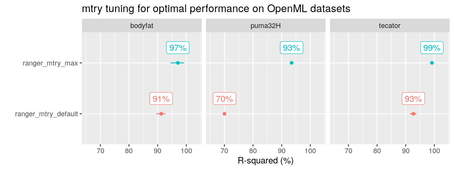

That tuning mtry for a Random Forest is important in the presence of many irrelevant features was already shown by Hastie et al. in their 2009 classic book “Elements of statistical Learning” (p615, Figure 15.7) (Hastie et al. 2009).

They showed that if mtry is kept at its default (square root of \(p\), the total number of features), as more irrelevant variables are added, the probability of the relevant features being selected for splitting becomes too low, decreasing performance. So for datasets with a large proportion of irrelevant features, mtry tuning (increasing its value) is crucially important.

Before we move on to RF feature selection, let’s see what else we can tune in RF apart from mtry.

RF tuning: what else can we tune?

With respect to the other RF parameters, a quick rundown:

I left the num.trees at its default (500), and chose “variance” as the splitrule for regression problems, and “gini” for classification problems (alternative is “extratrees” which implements the “Extremely Randomized Trees” method (Geurts, Ernst, and Wehenkel 2006) but I have yet to see convincing results that demonstrate ERT performs substantially better). I checked a few key results at lower and higher num.trees as well (100 and 1000 respectively): 100 is a bit low for the Out-of-bag predictions to stabilize, 500 appears to be a sweet spot, with no improvement in R-squared mean or a significant reduction in R2 variance between runs either.

I played around a bit with the min.node.size parameter, for which often the sequence 5,10,20 is mentioned to vary over. Setting this larger should reduce computation, since it leads to shorter trees, but for the datasets here, the effect is on the order of say 10% reduction, which does not warrant tuning it IMO. I left this at its default of 5 for regression and 1 for classification.

Finally, Marvin Wright points to results from Probst et al.(Probst, Wright, and Boulesteix 2019) that show sample.fraction to be an important parameter as well. This determines the number of samples from the dataset to draw for each tree. I have not looked into this, instead I used the default setting from ranger() which is to sample with replacement, and to use all samples for each tree, i.e sample.fraction = 1.

To conclude: we focus on mtry and leave the rest alone.

From RF tuning to RF feature selection

A natural question to ask is why not simply get rid of the irrelevant features? Why not perform feature selection?

The classic book Applied Predictive Modeling (Kuhn and Johnson 2013) contains a similar simulation experiment (on the solubility dataset, for RF I reproduce their results below) showing the negative effects of including many irrelevant features in a Random Forest model (chapter 18). And indeed, instead of tuning RF, they suggest removing the irrelevant features altogether, i.e. to perform feature selection. Also their follow up book on Feature engineering and selection by Kuhn & Johnson from 2019 (Kuhn and Johnson 2019) elaborates on this.

RF Feature selection

To perform feature selection, we use the recursive feature elimination (RFE) procedure, implemented for ranger in caret as the function rfe(). This is a backward feature selection method, starting will all predictors and in stepwise manner dropping the least important features (Guyon et al. 2002).

When the full model is created, a measure of variable importance is computed that ranks the predictors from most important to least. […] At each stage of the search, the least important predictors are iteratively eliminated prior to rebuilding the model.

— Pages 494-495, Applied Predictive Modeling, 2013.

(Computationally, I think it makes more sense to start with only the most relevant features and add more features in a stepwise fashion until performance no longer improves but reaches a plateau. But that would require writing my own “forward procedure”, which I save for another day.)

As this is a procedure that drops predictors that do not correlate with the outcome, we have to be extremely careful that we end up with something that generalizes to unseen data. In (Kuhn and Johnson 2013) they convincingly show that a special procedure is necessary, with two loops of cross validation first described by (Ambroise and McLachlan 2002). The outer loop sets aside one fold that is not used for feature selection (and optionally model tuning), whereas the inner loop selects features and tunes the model. See Chapter 10.4 of their follow up book (Kuhn and Johnson 2019) for detailed documentation and examples.

Typically, as we start removing irrelevant features, performs either stays constant or even increases until we reach the point where performs drops. At this point features that are predictive of the outcome are getting removed.

Note that we do not tune the mtry variable of RF in this procedure. Empirically, it has been observed that this either has no effect, or only leads to marginal improvements (Kuhn and Johnson 2019; Svetnik, Liaw, and Tong 2004). Conceptually, tuning (increasing) mtry is a way to reduce the effect of irrelevant features. Since we are applying a procedure to remove the irrelevant features instead, it makes sense that tuning has little benefit here.

(As I was curious, I nevertheless created a set of custom helper functions for rfe() that tune mtry during the feature selection procedure, see the RangerTuneFuncs.R script, results not shown)

So we expect that either tuning mtry , OR performing feature selection solves the problem of irrelevant variables. Indeed, this is also what we find on the three OpenML datasets. Both the RF tuning approach (Setting mtry at its maximum value) as well as the RF feature selection using RFE result in optimal performance:

plot_performance(data =fit_list %>% filter(ds_group == "openML"),
                 axis_label = "R-squared (%)",
                 plot_title = "mtry tuning vs feature selection for three OpenML datasets")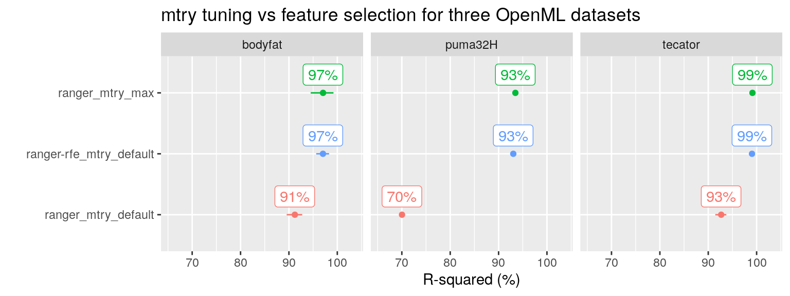

Can RF feature selection (“ranger-rfe” in the plot below) solve our problems with the “Friedman 1” simulated data as well?

plot_performance(data = fit_list %>% filter(ds_group == "df_friedman1"),
                 axis_label = "R-squared (%)",
                 plot_title = "Feature selection vs tuning on simulated data with noise added")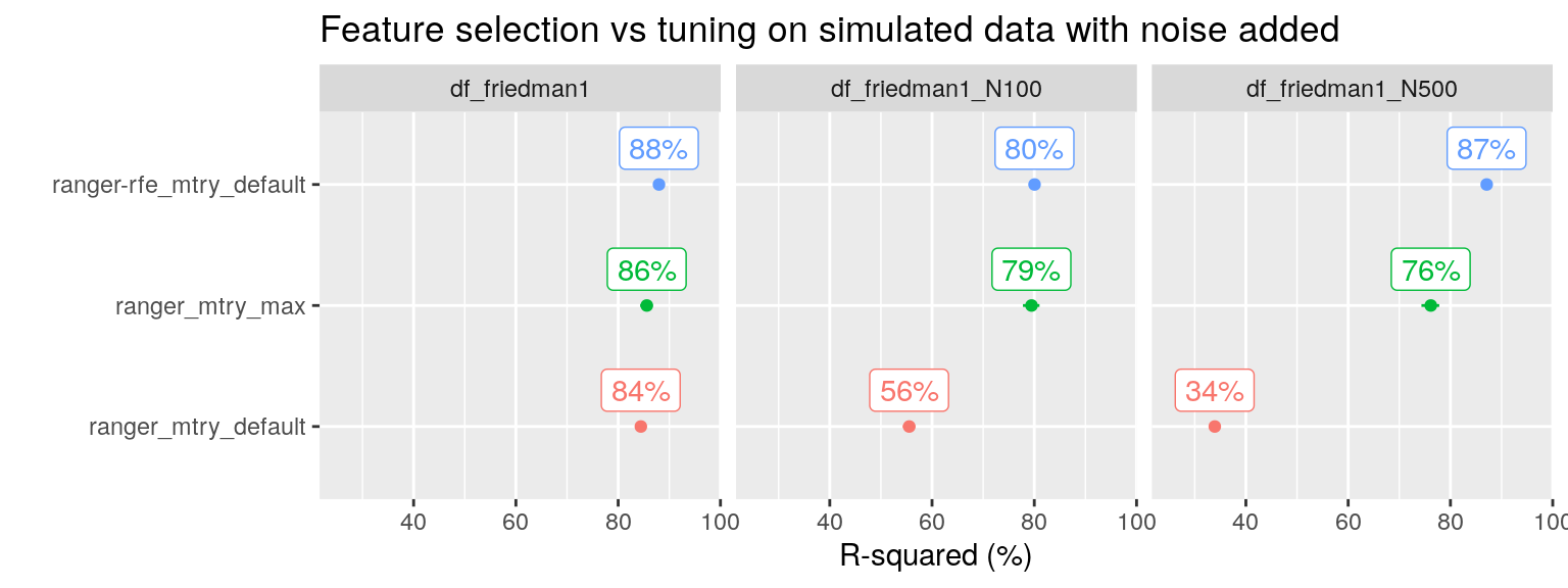

Yes, it can! And here we see that RF tuning is not enough, we really need to identify and remove the irrelevant variables.

N.b. For df_friedman1_N100, the RFE tuning grid is based on equidistant steps starting with \(p = 2\) and included as smallest values only \(p = 2\) and \(p = 14\), so it skipped the optimal value \(p = 5\). This explains the sub optimal performance for RFE with 105 noise variables added. For df_friedman1_N500, the tuning grid was exponential and included 2, 3, 6 and 12 (up to \(p = 510\)). The RFE procedure selected \(p = 6\) as optimal, this included as top five variables the five predictors that contained the signal.

A similar pattern is seen for the solubility dataset with noise added, an example taken from (Kuhn and Johnson 2013):

plot_performance(data = fit_list %>% filter(ds_group == "solubility" & ds_name != "solubility_N500_perm"),
                 axis_label = "R-squared (%)",
                 plot_title = "Feature selection vs tuning on Solubility data with noise added")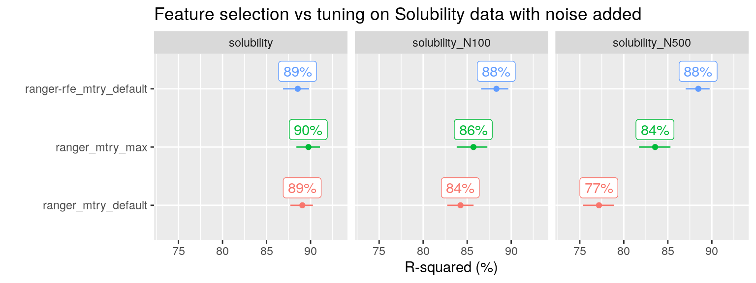

Note that on the original solubility dataset, neither tuning nor feature selection is needed, RF already performs well out of the box.

Doing it wrong: RF tuning after RFE feature selection on the same dataset

Finally, we echo others in stressing the importance of using a special nested cross-validation loop to perform the feature selection and performance assessment, especially when a test set is not available. “If the model is refit using only the important predictors, model performance almost certainly improves” according to Kuhn & Johnson (APM 2013). I also found a blog post [here] that references (Hastie et al. 2009) regarding the dangers when using both feature selection and cross validation.

To drive the point home, I have taken the solubility dataset with 500 noise predictors added (951 observation, with in total 228 + 500 = 728 predictors), and scrambled the \(y\) variable we wish to predict. With scrambling I mean shuffling the values of \(y\), thereby removing any correlation with the predictors. This is an easy way to check our procedure for any data leakage from the training set to the test set where we evaluate performance.

All three RF modeling approaches now correctly report an R-squared of approximately 0%.

plot_performance(fit_list %>% filter(ds_name == "solubility_N500_perm"),
                 axis_label = "R-squared (%)",
                 plot_title = "Feature selection vs tuning on simulated data after scrambling y") + expand_limits(y = 90)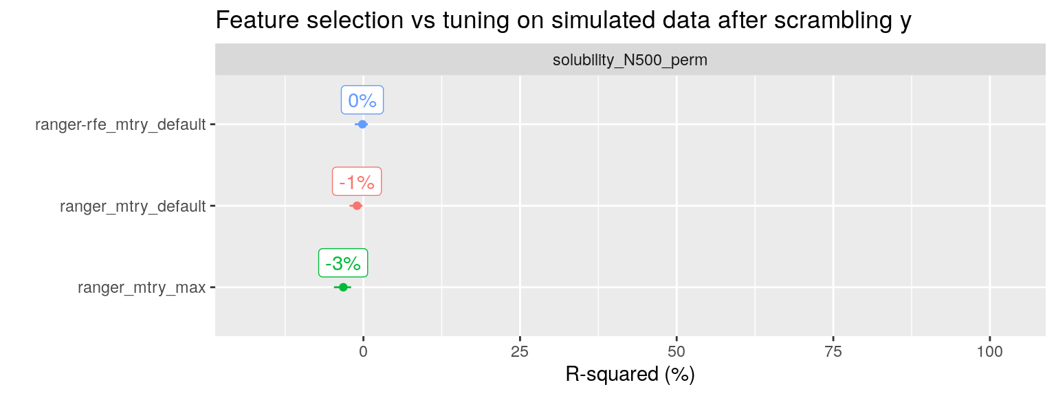

However, if we do RF tuning on this scrambled dataset, after we performed RFE feature selection, we get cross-validated R-squared values of 5-10%, purely based on noise variables “dredged” from the hundreds of variables we supplied to the algorithm. For full code see the R notebook on my Github

(Note that I had to play around a bit with the RFE settings to not have it pick either the model with all features or the model with only 1 feature: using RMSE as a metric, and setting pickSizeTolerance the procedure selected a model with 75 predictors. Retraining this model using caret::train gave me the result below)

trainObject <- readRDS("rf_rfe_post/post_rfe_train.rds")

trainObject

## Random Forest 
## 
## 951 samples
##  75 predictor
## 
## No pre-processing
## Resampling: Cross-Validated (10 fold) 
## Summary of sample sizes: 857, 855, 855, 856, 856, 858, ... 
## Resampling results across tuning parameters:
## 
##   mtry  RMSE      Rsquared    MAE     
##    1    2.001946  0.07577078  1.562253
##    2    1.997836  0.06977449  1.558831
##    3    1.993046  0.07166917  1.559323
##    5    1.983549  0.08801892  1.548190
##    9    1.988541  0.06977760  1.551304
##   15    1.987132  0.06717113  1.551576
##   25    1.989876  0.06165605  1.552562
##   44    1.985765  0.06707004  1.550177
##   75    1.984745  0.06737729  1.548531
## 
## Tuning parameter 'splitrule' was held constant at a value of variance
## 
## Tuning parameter 'min.node.size' was held constant at a value of 5
## RMSE was used to select the optimal model using the smallest value.
## The final values used for the model were mtry = 5, splitrule = variance
##  and min.node.size = 5.

This illustrates the dangers of performing massive variable selection exercises without the proper safeguards. Aydin Demircioğlu wrote a paper that identifies several radiomics studies that performed cross-validation as a separate step after feature selection, and thus got it wrong (Demircioğlu 2021).

Conclusions

To conclude: we have shown that for in the presence of (many) irrelevant variables, RF performance suffers and something needs to be done. This can be either tuning the RF, most importantly increasing the mtry parameter, or identifying and removing the irrelevant features using the RFE procedure rfe() part of the caret package in R. Selecting only relevant features has the added advantage of providing insight into which features contain the signal.

Interestingly, on the “real” datasets (openML, the solubility QSAR data) both tuning and feature selection give the same result. Only when we use simulated data (Friedman1), or if we add noise to real datasets (iris, solubility)) we find that mtry tuning is not enough, and removal of the irrelevant features is needed to obtain optimal performance.

The fact that tuning and feature selection are rarely compared head to head might be that both procedures have different implicit use cases: ML tuning is often performed on datasets that are thought to contain mostly relevant predictors. In this setting feature selection does not improve performance, as it primarily works through the removal of noise variables. On the other hand, feature selection is often performed on high-dimensional datasets where prior information is available telling us that relatively few predictors are related to the outcome, and the many noise variables in the data can negatively influence RF performance.

N.b. As is often the case with simulation studies, an open question is how far we can generalize our results. (Svetnik et al. 2003) identified a classification dataset Cox-2 that exhibits unexpected behavior: The dataset gives optimal performance with mtry at its maximum setting, indicative of a many irrelevant predictors, so we expect feature selection to find a smaller model that gives the same performance at default mtry. However, surprisingly, performance only degraded after performing feature selection using RFE. I wrote the authors (Vladimir Svetnik and Andy Liaw) to ask for the dataset, unfortunately they suffered a data loss some time ago. They obtained the data from Greg Kauffman and Peter Jurs (Kauffman and Jurs 2001), I reached out to them as well but did not receive a reply.

Acknowledgements: I’d like to thank Philipp Probst and Anne-Laure Boulesteix for their constructive comments and suggestions on this blog post.